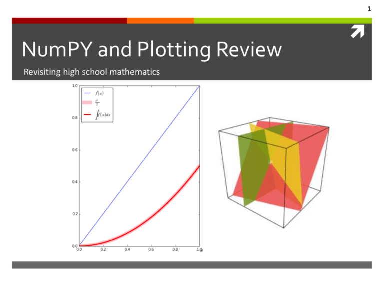
1
NumPY and Plotting Review
Revisiting high school mathematics

2
Module
 Python module is a collection of functions to support
specialized tasks.
 To use an external module, let Python import the module
by name
 A Python script can be a module.
3
My First Module
•
‘myclass’ module
•
Functions for set operations
•
Functions for plotting
•
Functions for counting

4
NumPY
 NumPY = Numerical Python
 Support vectorized operations

Most of NumPY function calls are basically mapping.

Most of NumPY functions take a list, a tuple, or a
NumPY.array()

Easy support for parallel computing  Fast!
5
NumPY
 Basic Data Structure: a improved counter part of a list

NumPY.array()

Support all basic operations such as +, -, *, /, **, %

Every basic operation works element-wise
 The construction of a list: [ 1,2,3,4 ]
The construction of a tuple: ( 1,2,3,4 )
The construction of a np.array:
numpy.array([1,2,3,4]) or numpy.array((1,2,3,4))
6
Recitation For NumPY array

7
NumPY array and matrix
print np.array([1,2,3])
print np.array([[1,2],[3,4]])
 NP.array() supports multi-dimensional array
 NP.dot() for multiplication between vectors and matrices
 NP.linalg.inv() to compute the inverse of a matrix.
http://docs.scipy.org/doc/numpy/reference/generated/numpy.dot.html#numpy.dot
http://docs.scipy.org/doc/numpy/reference/generated/numpy.linalg.inv.html
8
NumPY Documentation
 http://docs.scipy.org/doc/numpy/genindex.html
np.dot(); the inner product, multiplication between
matrices
np.linalg.inv()
…
many useful functions
 http://docs.scipy.org/doc/numpy/user/basics.html
Numpy Basics!
9
Recitation For Basic Geometry

10
The ‘mygeom’ module
 A module contains functions related to basic geometry
mostly about a line graph.

Drawing a graph with basic parameters such as slope
and intercept

Drawing a graph perpendicular to a given line equation

Computing the intersection of two lines

Measuring the distance between a point and a line
equation

Computing a line from a scattered data (Linear
Regression)
11
Line Graph
 A line is a set of points which doesn’t change its direction.
 The definition of a line in Mathematics
1) Using a parametric formula,
A line is specified by the parameter x and its output y
2) Using an implicit formula,
From the domain of x and y, the equation specified the set of x
and y which satisfies the equation.
 The difference is its domain.
12
Parametric Line Equation
 The slope and intercept
 A line between two points is given as
 Why?
By subtraction
 The slope and the intercept are
13
Intersection of two lines

14
Linear System
 System of linear equations.

Wikipedia Example
16
Linear System to Matrix
 Move all x and y to the left and factor terms w.r.t x and y
 Move all constants to the right
17
Linear System to Matrix
 Move all x and y to the left and factor terms w.r.t x and y
 Move all constants to the right
18
The inverse
19
20
The ‘mygeom’ module
 A module contains functions related to basic geometry
mostly about a line graph.

Drawing a graph with basic parameters such as slope
and intercept

Drawing a graph perpendicular to a given line equation

Computing the intersection of two lines

Measuring the distance between a point and a line
equation

Computing a line from a scattered data (Linear
Regression)
21
Measuring the distance between 
a point and a line
22
Distance between a point and a line
 In many applications, linear regression for example, the
distance between a point and a line is used as an
important measure.
 Let’s see an example,
23
Distance between a point and a line
 The plot is drawn as below and its distance is
24
Distance between a point and a line
1. Find a graph perpendicular Lp to the graph given L, which
passes through the given point p
2. Find the intersection q from L and Lp
25
Distance between a point and a line

Finding the intersection and computing the distance between those
two points are complicated!
 Different approach with the implicit form of a line equation,
The
is called the directional vector of the line.
 Its normal vector, perpendicular to the directional vector is given as
26
The Inner Product

The definition of the inner product between two vectors
is defined as

From the definition of the trigonometric function,

The geometric interpretation
assuming u is a unit vector,
27
Recitation for the System of
Linear Equations

28
The inverse
29
Recitation for the System of
Linear Equations

30
Root Finding

31
Root Finding
 One of Classic Problems
32
Root Finding
 Based on high school knowledge
33
Linear Search
 From the beginning value up to the limit,
def find_root(fun, h, begin, limit):
x = float(begin)
while np.fabs(fun(x)) >= 1e-6 and x < limit:
x=x+h
return (x < limit, np.round(x,5))
34
Linear Root Finding
35
Linear Search vs. Binary Search
O(n) vs. O(log n)
We should do better!
36
Binary Search with Real Numbers
 Exactly same algorithm.
 Instead of using a list and its index, use a math function
and compare f(x) == 0.
 Considering numerical error, find x such that
 If f(x) < 0, go up;
Otherwise, f(x) > 0, go down.
37
Bisection Algorithm
38
Basic Numerical Methods
• Numerical Derivatives
• Numerical Integration

39
Derivatives
 The derivative operation is to compute the change of a
function informally.
 With a computer,
def dfunc(func, x, h):
return (f(x+h) – f(x)) / h
40
Vectorized Operations
 Use numpy.array() instead of a list or a tuple because of
this.
 Every basic operator, +,-,*,/ works in parallel or in an
element-wise manner.
 No need to use list comprehension.
41
Recitation for Numerical
Differentiation

42
Numerical Integration
 Integrating a function
 How can we compute f(x) from f’(x)?

For example,
 We know f’(x) and h.
43
Numerical Integration
 Playing with the derivative equation,
 If we know f(x), for example, f(0), the rest of f(x) can be
successively computed
44
Numerical Integration
 Initial value problem (IVP)

Given initial conditions and differential equations, identify
the integral function.
 We focus on simple integration.
 Further mathematics is taught in Math661 or Math662
classes; or Real Analysis, Numerical Analysis, Scientific
Programming, Calculus 2 or 3
45
Numerical Integration

Our goal is to find a function which satisfies

Assume h, x0, and f(x0) are given


h=0.001, x0=0, f(x0) = 0
how many loops required to compute f(1)?

It is amount to 1/(1e-3) = 1000 iterations.
46
Numerical Integration
 A computer cannot deal with a continuous function.
 Convert the equation into a number of sequences
 Sample the derivative function at points of the sequence
Discretization Process
47
Numerical Integration
 Discretization Process

Construct a recurrence relationship
Discretization Process
fx = fx + h*cos(x0+jh)
fx[j+1] = fx[j] + h*cos(x0+jh)
48
Recitation for Numerical
Integration

49
The Inner Product
50
My Approach
 The distance between a point and a line can be found by
solving an equation.
 Combining an equation of circle and a line graph into a
single equation in an implicit form, whose positive root is
the distance from the point and the line.
51
Line and Point
 The distance between a line and a point is given as a
closed form solution.