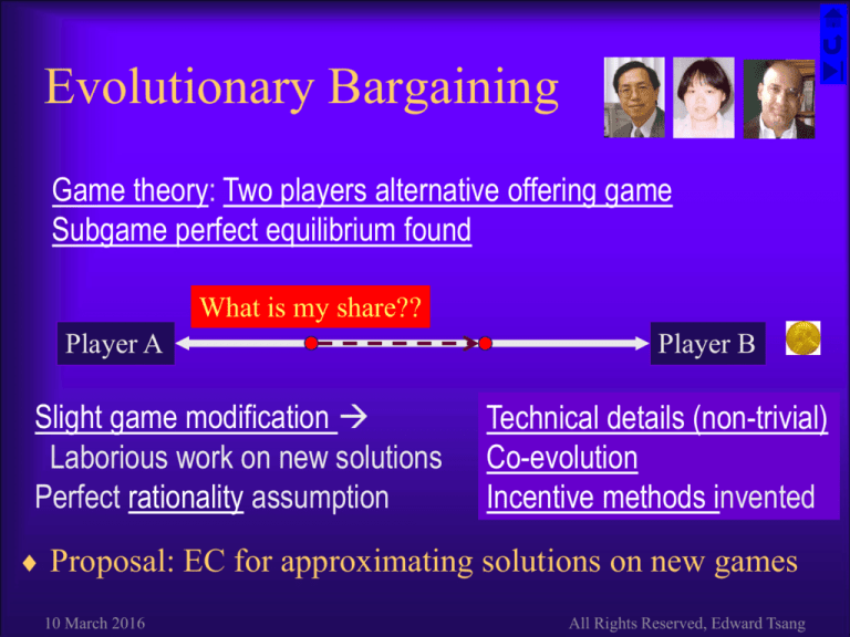
Evolutionary Bargaining
Game theory: Two players alternative offering game
Subgame perfect equilibrium found
What is my share??
Player A
Slight game modification
Laborious work on new solutions
Perfect rationality assumption
Player B
Technical details (non-trivial)
Co-evolution
Incentive methods invented
Proposal: EC for approximating solutions on new games
10 March 2016
All Rights Reserved, Edward Tsang
Evolutionary Bargaining Conclusions
Demonstrated GP’s flexibility
– Models with known and unknown solutions
– Outside option
– Incomplete, asymmetric and limited information
Co-evolution is an alternative approximation method
to find game theoretical solutions
– Perfect rationality assumption relaxed
– Relatively quick for approximate solutions
– Relatively easy to modify for new models
Genetic Programming with incentive / constraints
– Constraints helped to focus the search in promising spaces
Lots remain to be done…
10 March 2016
All Rights Reserved, Edward Tsang
Two players alternative offering game
Player 1: How about 70% for me 30% for you?
t = 0, Player 1’s pay off isPlayer
70% 2: No, I want 60%
Player 1: No, how about 50-50?
Player
No,
I want
least
55%
t = 2, Player 1’s pay
off is2:50%
e0.1 at2 =
41%
If neither players have any incentive to compromise,
this can go on for ever
Payoff drops over time – incentive to compromise
A’s Payoff = xA exp(– rA tΔ)
Let r1 be 0.1, Δ be 1
10 March 2016
All Rights Reserved, Edward Tsang
Payoff decreases over time
Decrease of utility over time
Player's Share
1.2
r=0.1
1
0.2
0.8
0.3
0.4
0.6
0.5
0.4
0.6
0.2
0.7
0.8
0
0
1
2
3
4
5
Time
10 March 2016
6
7
8
9
10
0.9
1.0
All Rights Reserved, Edward Tsang
Bargaining in Game Theory
by
A’s Payoff = xA exp(– rA tΔ)
Important Assumptions:
– Both players rational
– Both players know everything
Equilibrium solution for A:
A = (1 – B) / (1 – AB)
where i = exp(– ri Δ)
10 March 2016
0
?
xA
xB
A
B
Decay of Payoff over time
0.6
0.5
0.4
Payoff
Rubinstein 1982 Model:
In
=reality:
Cake to share between A and B
(=Offer
1)
at time t = f (rA, rB, t)
A and
B make alternate offers
Is
it necessary?
xA = A’s share
(xB = – xA)
Is
it
rational?
(What
is rational?)
rA = A’s discount rate
t = # of rounds, at time Δ per round
A’s payoff xA drops as time goes
0.3
0.2
0.1
0.0
Time t
0
1
Optimal offer:
xA = A
at t=0
2
3
4
5
6
7
8
9
10
Notice:
No time t here
All Rights Reserved, Edward Tsang
Evolutionary Computation
for Bargaining
Technical Details
Issues Addressed in EC for Bargaining
Representation
– Should t be in the language?
One or two population?
How to evaluate fitness
– Fixed or relative fitness?
How to contain search space?
Discourage irrational strategies:
– Ask for xA>1?
– Ask for more over time?
– Ask for more when A is low?
/
1
B
1
A
Details of GP
10 March 2016
All Rights Reserved, Edward Tsang
B
Two populations – co-evolution
We want to deal with
Player 1
Player 2
…
…
…
…
asymmetric games
– E.g. two players may have
different information
One population for training
each player’s strategies
Co-evolution, using relative
fitness
– Alternative: use absolute fitness
Evolve over time
10 March 2016
All Rights Reserved, Edward Tsang
Representation of Strategies
A tree represents a mathematical function g
Terminal set: {1, A, B}
Functional set: {+, , ×, ÷}
Given g, player with discount rate r plays at time t
g × (1 – r)t
Language can be enriched:
– Could have included e or time t to terminal set
– Could have included power ^ to function set
Richer language larger search space harder
search problem
10 March 2016
All Rights Reserved, Edward Tsang
Incentive Method:
Constrained Fitness Function
No magic in evolutionary computation
– Larger search space less chance to succeed
Constraints are heuristics to focus a search
– Focus on space where promising solutions may lie
Incentives for the following properties in the function
returned:
– The function returns a value in (0, 1]
– Everything else being equal, lower A smaller share
– Everything else being equal, lower B larger share
Note: this is the key to search effectiveness
10 March 2016
All Rights Reserved, Edward Tsang
Incentives for Bargaining
F(gi) =
GF(s(gi)) + B
If gi in (0,1] &
B ≥ 3 (tournament selection is used) SMi > 0 & SMj > 0
GF(s(gi)) + ATT(i) + ATT(j) If gi in (0,1] &
(SMi ≤ 0 or SMj ≤ 0)
ATT(i) + ATT(j) – e(–1/|gi|)
If gi NOT in (0,1]
GF(s(gi)) is the game fitness (GF) of a strategy (s) based on the
function gi, which is generated by genetic programming
When gi is outside (0, 1], the strategy does not enter the games;
the bigger |gi|, the lower the fitness
10 March 2016
All Rights Reserved, Edward Tsang
C1: Incentive for Feasible Solutions
The function returns a value in (0, 1]
The function participates in game plays
The game fitness (GF) is measured
A bonus (B) incentive is added to GF
– B is set to 3
– Since tournament is used in selection, the absolute
value of B does not matter (as long as B>3)
10 March 2016
All Rights Reserved, Edward Tsang
f
C2: Incentive for Rational A
Everything else being equal, lower A smaller share
for A
Given a function gi:
The sensitive measure SMi(i, j, α) measures how
much gi decreases when i increases by α
1
Attribute ATT(i) =
If SMi(i, j, α) > 1
e –(1/ SMi(i, j, α)) If SMi(i, j, α) ≤ 1
0 < ATT(i) ≤ 1
10 March 2016
All Rights Reserved, Edward Tsang
f
C3: Incentive for Rational B
Everything else being equal, lower B larger share
for A
Given a function gi:
The sensitive measure SMj(i, j, α) measures how
much gi increases when j increases by α
Attribute ATT(j) =
1
If SMj(i, j, α) > 1
e–(1/ SMj(i, j, α))
If SMj(i, j, α) ≤ 1
0 < ATT(j) ≤ 1
10 March 2016
All Rights Reserved, Edward Tsang
f
Sensitivity Measure (SM) for i
SMi(i, j, α) =
[gi(i (1 + α), j) gi(i, j)]
÷ gi(i, j)
If i (1 + α) < 1
[gi(i, j) gi(i (1 α), j)]
÷ gi(i, j)
If i (1 + α) 1
SMi measures the derivatives of gi -- how much gi
decreases when i increases by α
(gi is the function which fitness is to be measured)
10 March 2016
All Rights Reserved, Edward Tsang
f
Sensitivity Measure (SM) for j
SMj(i, j, α) =
[gi(i, j) gi(i, j (1 + α))] If j (1 + α) < 1
÷ gi(i, j)
[gi(i, j (1 α)) gi(i, j)] If j (1 + α) 1
÷ gi(i, j)
SMj measures the derivatives of gi -- how much gi
increases when j increases by α
(gi is the function which fitness is to be measured)
10 March 2016
All Rights Reserved, Edward Tsang
f
Bargaining Models Tackled
Determin
ants
Discount
Factors
Complete
Information
* Rubinstein 82
+ Outside * Binmore 85
Options
Uncertainty
1-sided
2-sided
* Rubinstein 85 x Bilateral
x Imprecise info ignorance
Ignorance
x Uncertainty +
More could be
Outside Options done easily
* = Game theoretical solutions known
x = game theoretic solutions unknown
10 March 2016
All Rights Reserved, Edward Tsang
Models with known equilibriums
Complete Information
Rubinstein 82 model:
– Alternative offering, both A and B know A & B
Binmore 85 model, outside options:
– As above, but each player has an outside offer, wA and wB
Incomplete Information
Rubinstein 85 model:
– B knows A & B
– A knows A
– A knows B is w with probability w0, s (> w) otherwise
10 March 2016
All Rights Reserved, Edward Tsang
Models with unknown equilibriums
Modified Rubinstein 85 / Binmore 85 models:
1-sided Imprecise information
– B knows A & B; A knows A and a normal
distribution of B
1-sided Ignorance
– B knows both A and B; A knows A but not B
2-sided Ignorance
– B knows B but not A; A knows A but not B
Rubinstein 85 + 1-sided outside option
10 March 2016
All Rights Reserved, Edward Tsang
Equilibrium with Outside Option
xA*
Conditions
A
wA A A
wB B B
1 wB
wAA(1wB)
wB > B B
BwA+(1B)
wA > A A
wBB(1wA)
1 wB
wA
10 March 2016
wA>A(1wB) wB>B(1wA)
wA+ wA > 1
–
All Rights Reserved, Edward Tsang
Equilibrium in Uncertainty – Rub85
1 s
Vs
1 1 s
w0 < w*
w0 > w*
2 = w
x1*
t*
Vs
0
xw0
0
2
V
Vs
*
s
1
w
1 w 1Vs w 1
10 March 2016
x w0
2 = s
x1*
Vs
1 – ((1 –
xw0) / w)
t*
0
1
1 w 1 12 1 w0
1 2 1 w0 1 w w0
1
All Rights Reserved, Edward Tsang
Running GP in Bargaining
Representation, Evaluation
Selection, Crossover, Mutation
Representation
Given A and B, every tree represents a
constant
/
+
1
B
1
A
10 March 2016
A
B
1
A
1
B
All Rights Reserved, Edward Tsang
Population Dynamics
Player 1
Population of
strategies
Player 2
Evaluate
Fitness
Population of
strategies
Select,
Crossover,
Mutation
Select,
Crossover,
Mutation
New
Population
New
Population
10 March 2016
All Rights Reserved, Edward Tsang
Evaluation
Given the discount factors, each tree is
translated into a constant x
– It represents the demand represented by the tree.
All trees where x < 0 or x > 1 are evaluated
using rules defined by the incentive method
All trees where 0 x 1 enter game playing
Every tree for Player 1 is played against every
tree for Player 2
10 March 2016
All Rights Reserved, Edward Tsang
Evaluation Through Bargaining
Player 1 Demands
Demands by Player 2’s strategies
Player 1
.20 Fitness
.75
0.75
.46
.31
.65
.75
0
0
0
.24
.24
.24
.24
.24
0.96
.36
.36
.36
0
.36
1.08
.59
0
.59
0
.59
1.18
Incentive method ignored here for simplicity
10 March 2016
All Rights Reserved, Edward Tsang
Selection
Rule (Demand)
Fitness
Normalized
Accumulated
R1 (0.75)
0.75
0.19
0.19
R2 (0.96)
0.96
0.24
0.43
R3 (1.08)
1.08
0.27
0.70
R4 (1.18)
1.18
0.30
1.00
3.97
1
Sum:
A random number r between 0 and 1 is generated
If, say, r=0.48 (which is >0.43), then rule R3 is selected
10 March 2016
All Rights Reserved, Edward Tsang
/
Crossover
Parents
B
1
1
A
/
1
1
A
B
1
+
A
A
B
1
A
10 March 2016
Offspring
B
+
B
1
A
1
B
All Rights Reserved, Edward Tsang
Mutation
+
A
B
+
1
A
B
1
A
A
/
B
B
1
A
With a small probability, a branch (or a node)
may be randomly changed
10 March 2016
All Rights Reserved, Edward Tsang
Discussions on Bargaining
http://cswww.essex.ac.uk/CSP/bargain
