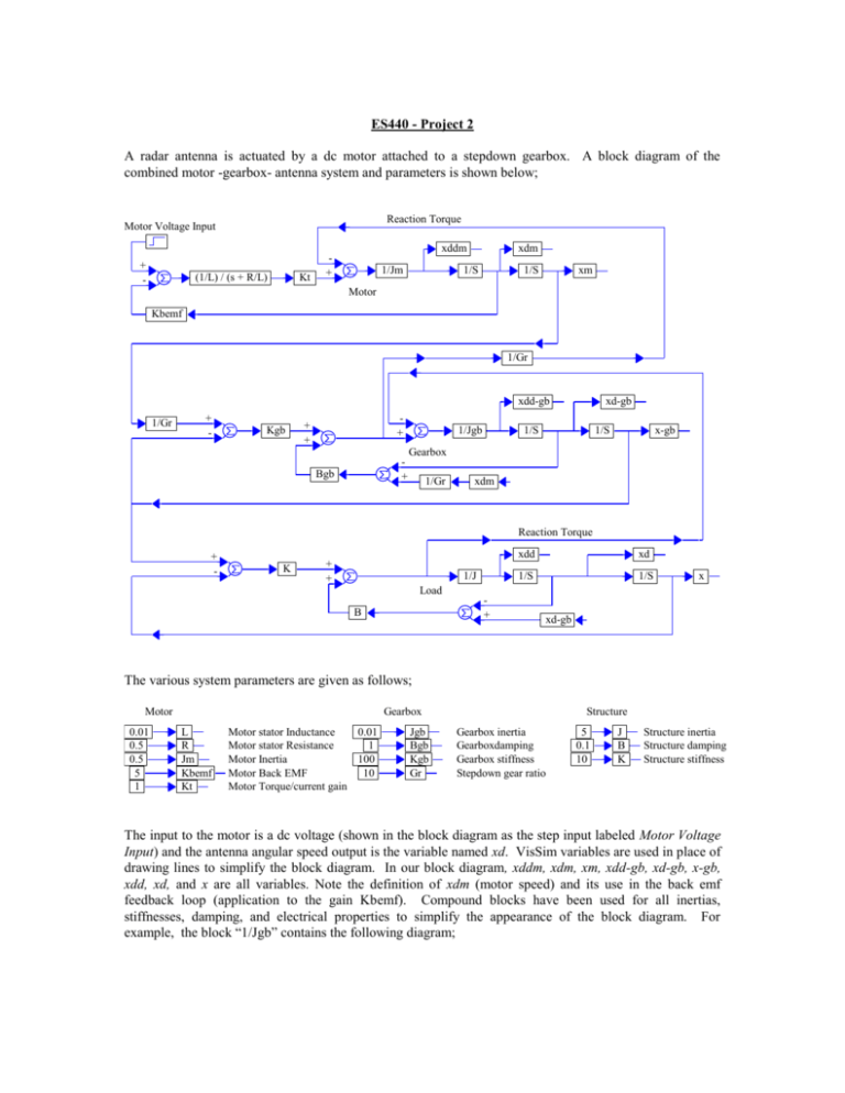
ES440 - Project 2
A radar antenna is actuated by a dc motor attached to a stepdown gearbox. A block diagram of the
combined motor -gearbox- antenna system and parameters is shown below;
Reaction Torque
Motor Voltage Input
+
-
(1/L) / (s + R/L)
Kt
xddm
+
1/Jm
xdm
1/S
1/S
xm
Motor
Kbemf
1/Gr
xdd-gb
1/Gr
+
-
Kgb
+
+
+
+
Bgb
1/Jgb
xd-gb
1/S
1/S
x-gb
Gearbox
1/Gr
xdm
Reaction Torque
+
-
K
+
+
1/J
xdd
xd
1/S
1/S
x
Load
+
B
xd-gb
The various system parameters are given as follows;
Motor
0.01
0.5
0.5
5
1
Gearbox
L
R
Jm
Kbemf
Kt
Motor stator Inductance
0.01
Motor stator Resistance
1
Motor Inertia
100
Motor Back EMF
10
Motor Torque/current gain
Jgb
Bgb
Kgb
Gr
Structure
Gearbox inertia
Gearboxdamping
Gearbox stiffness
Stepdown gear ratio
5
0.1
10
J
B
K
Structure inertia
Structure damping
Structure stiffness
The input to the motor is a dc voltage (shown in the block diagram as the step input labeled Motor Voltage
Input) and the antenna angular speed output is the variable named xd. VisSim variables are used in place of
drawing lines to simplify the block diagram. In our block diagram, xddm, xdm, xm, xdd-gb, xd-gb, x-gb,
xdd, xd, and x are all variables. Note the definition of xdm (motor speed) and its use in the back emf
feedback loop (application to the gain Kbemf). Compound blocks have been used for all inertias,
stiffnesses, damping, and electrical properties to simplify the appearance of the block diagram. For
example, the block “1/Jgb” contains the following diagram;
Where “Jgb” is the variable defined to be the gearbox inertia. Other compound blocks in the diagram are
constructed similarly.
Section I:
1. Compute the transfer function of xd / Motor Voltage Input analytically (using block diagram
manipulations) showing all work. Hint: the closed loop transfer function, zeros, and poles should be;
T ( s)  40
s 3  200 s 2  10000 s
s 7  160.04 s 6  17508.2 s 5  660770.1s 4  11048008s 3  1500200 s 2  20000000 s
Zeros:
0
100
100
Poles:
0
55.01  j 89.309
24.995  j19.361
1.364e  2  j1.348
2. Check your transfer function by first coding the model in VisSim and then numerically obtain the
transfer function (analyze…transfer function info). Use the following simulation information: Range Start =
0, Step Size = . 0.0025, Range End = 25, Integration Algorithm = Runge Kutta 4th order.
3.
What are the poles, zeros, DC gain (you may use vissim for this).
4. Derive an approximate second order transfer function with the correct DC gain using the approximating
method outlined in class. You may use a damping ratio of 0 for this approximation.
5. Compare the results of the true and approximate transfer function by applying a unit step input to each
(in VisSim) and plot the xd outputs on one plot. Use the following simulation information: Range Start = 0,
Step Size = . 0.0025, Range End = 25, Integration Algorithm = Runge Kutta 4th order.
Section II:
.0363
, you will design and test (via simulation) a
s  1.817
feedback controller which will achieve the following design specifications:
Using the approximate transfer function: G ( s) 
1.
2.
3.
4.
2
System is stable
Steady State Unit Step Error = 0
Steady State Unit Ramp Error <= 0.4
Damping Ratio >=0.5
5.
Settling Time < 12 seconds
After the controller has been designed and tested on the approximate transfer function you will compare its
performance (via simulation) on the actual full order system from Section I.
The controller is designed in two steps; (1) an inner loop and (2) an outer loop. The purpose of the inner
loop controller is to modify the transient response of the plant using a cascade lead compensator to move
the plant poles leftward making the inner loop feedback system faster and more stable. To the outer loop,
the closed inner loop will look like a gain over the frequency range of the outer loop. The outer loop
controller, consisting of an integral control, will slightly modify the transient response of the closed inner
loop, but more importantly, will satisfy the two steady state error specifications (and maintain stability).
Perform the following steps, hand in all hand calculations, sketches, and computer results.
s  4.8
, in cascade with the G (s) in the
s  100
forward loop. Use a Root Locus sketch to design K Lead such that the dominant closed loop poles lie
near s1,2  5.29  j 5.26 . What is K Lead ? What are the resulting closed loop poles and zeros for the
inner loop?
1.
Add a lead compensator of the form, GLead (s)  K Lead  20.8 
2.
Code the closed inner loop in VisSim (using the approximate transfer function) and simulate it using a
stepsize of .0025, range end of 5 seconds and RK2 integration. These values will be used for the
remaining steps of the project. Plot the unit step response, unit ramp response, steady state unit step
error and the steady state unit ramp error.
3.
K
Add an integral compensator of the form, G int (s)  int , in cascade with the closed inner loop. Find
s
K int using a root locus sketch to place the dominant closed loop poles to satisfy the settling time
specification and the steady state ramp error specification. Your K int value should produce a dominant
pole pair near s1,2  4  j 7 with a damping of just under 0.5. What are the resulting closed loop
poles and zeros for the closed outer loop? What is the steady state step error coefficient and the steady
state ramp error coefficient?
4.
Code the closed outer loop in VisSim around the closed inner loop from part 2 and simulate it using a
stepsize of .0025, range end of 5 seconds and RK2 integrator. Plot the unit step response, unit ramp
response, steady state unit step error and the steady state unit ramp error. How do the error values
relate to the coefficient calculations made in part 3?
5.
Implement the controller (both inner and outer loops) on the original high order system (Section I) and
compare unit step responses between it and the reduced order (design) system. Plot the steady state
step and ramp errors also. Comment on differences in the responses.