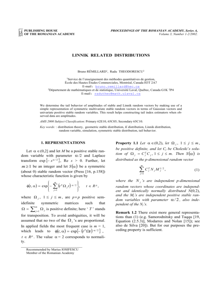
PUBLISHING HOUSE
OF THE ROMANIAN ACADEMY
PROCEEDINGS OF THE ROMANIAN ACADEMY, Series A,
Volume 3, Number 1-2/2002.
LINNIK RELATED DISTRIBUTIONS
Bruno RÉMILLARD1, Radu THEODORESCU2
1Service de l’enseignement des méthodes quantitatives de gestion,
École des Hautes Études Commerciales, Montréal, Canada H3T 2A7
E-mail: bruno.remillard@hec.ca
2Département de mathématiques et de statistique, Université Laval, Québec, Canada G1K 7P4
E-mail: radutheo@math.ulaval.ca
We determine the tail behavior of amplitudes of stable and Linnik random vectors by making use of a
simple representation of symmetric multivariate stable random vectors in terms of Gaussian vectors and
univariate positive stable random variables. This result helps constructing tail index estimators when observed data are amplitudes.
AMS 2000 Subject Classification: Primary 62E10, 65C05; Secondary 65C10.
Key words: : distribution theory, geometric stable distribution, K distribution, Linnik distribution,
random variable, simulation, symmetric stable distribution, tail behavior.
1. REPRESENTATIONS
Property 1.1 Let   (0,2), let Ω j , 1  j  m ,
Let   (0,2] and let M be a positive stable random variable with parameter  /2 and Laplace
transform exp  s  / 2 , Re s > 0. Further, let
be positive definite, and let Cj be Choleski’s solution of  j  C Tj C j , 1  j  m. Then S   is
m  1 be an integer and let S   be a symmetric
(about 0) stable random vector (Press [16, p.158])
whose characteristic function is given by


t ,    exp


 t
m
j 1
T
 jt


,


/2 
 

symmetric
m
j 1
matrices
tR ,
such
that
 j is positive definite; here ‘ T ’ stands
for transposition. To avoid ambiguities, it will be
assumed that no two of the  j ’s are proportional.
In applied fields the most frequent case is m = 1,
which leads to t ,   exp t T t   / 2  ,
t  R p . The value  = 2 corresponds to normality.
______________________________
Recommended by Marius IOSIFESCU
Member of the Romanian Academy
m
C
T
j
N j M 1j / 2 ,
(1)
j 1
where the N j ’s are independent p-dimensional
p
where Ω j , 1  j  m , are p  p positive semidefinite
distributed as the p-dimensional random vector
random vectors whose coordinates are independent and identically normally distributed N(0,2),
and the Mj’s are independent positive stable random variables with parameter  / 2 , also independent of the Nj’s.
Remark 1.2 There exist more general representations than (1) (e.g. Samorodnitsky and Taqqu [19,
Equation (2.5.3)], Modarres and Nolan [15]); see
also de Silva [20]). But for our purposes the preceding property is sufficient.
Bruno RÉMILLARD, Radu THEODORESCU
2. SIMULATION
For the normal case (  = 2) there exist simulation algorithms.
Property 1.1 leads to a simulation algorithm for
symmetric stable random vectors by making use of
positive univariate stable random variables. Next,
we can generate a positive stable random variable
by the method proposed by Chambers, Mallows,
and Stuck [4] that relies on results in Ibragimov
and Chernin [7] and Kanter [12].
Another algorithm for generating a three dimensional symmetric stable random vector is to be
found in Uchaikin and Gusarov [21]. A comparative simulation based study of the algorithms in [9]
and [21] was done by Boucher [3], who showed
the advantages of that in [9].
Since we know how to simulate univariate/multivariate symmetric stable random variables, we are also able to simulate univariate/multivariate Linnik random variables using
univariate positive stable random variables.
Devroye [5] provided a simple and elegant algorithm for simulating univariate Linnik random
variables. In Jacques, Rémillard and Theodorescu
[9, p. 217] we indicated an algorithm for the multivariate symmetric case, based on Property 1.1. Recall that for   (0,2] ,   0 , and the same
 j ’s, the characteristic function of the multivariate Linnik distribution is given by


t , ,   1 







tT  jt

j 1

m

/2



 ,


t  R p.
The associated probability density function will
depend on x via x T  1 x . For the case  = 2
(which is widespread in applied fields) and m = 1,
we obtain after some manipulations and for
x  R p the probability density function
f  x,   
1
2 p 1  p / 2 det  
 x T  1 x 




2


1/ 2
 p / 2
K  p / 2


2
If G(  ) is a gamma (  ,1) random variable independent of S(  ), then the characteristic function
of the random vector:
L,   S    G
1/ 
is (t , , ) . Consequently, the simulation of
L(  ,  ) amounts to the simulation of S   and
G(  ). We also mention the algorithm in Kozubowski [13].
3.TAIL BEHAVIOR
For  > 0 we consider the family of all random
variables X for which the tail property
lim x  P X  x   c
x 
holds, where c is a positive constant, generally
depending on  and possibly on other parameters.
According to Mandelbrot [14], we refer to it as the
Paretian family of index  . For   (0,2), stable
random variables (symmetric or not) are Paretian,
from which we conclude (Jacques, Rémillard, and
Theodorescu [9, pp. 214-216]) that Linnik random
variables are also Paretian.
We now assume that m = 1. We consider the
amplitudes (Euclidean norms) |S   | and
|L(  ,  )|. In certain applications, the only observed data are such quantities. This is the case in
particular for satellite and radar data (Anastassopoulos et al. [1] and Raghavan [18]).
Next, we examine the tail behavior of these
amplitudes. The following property complements
previous results obtained by Jacques, Rémillard,
and Theodorescu [9].
Property 3.1 Let   (0,2) and q  1 . We denote
by V j  x,   the expression
 sin j / 2.

x T  1 x ,
which involves the modified Bessel function K 
of the second kind of order  . The last expression
clearly links Linnik distributions to K  functions.
1
 1 j 1  j / 2 x  j E N

j!
j
We have


lim x q P S    x  
x 


and


 V x,   0
q
j
j 1

(2)
3
Linnik related distributions
lim x
q
x 


P L,   x  




W j x,    0

j 1

q

(3)
where
W x,    V x,  (  j ) / (),
j
j
and N is a p-dimensional centered Gaussian vector with covariance matrix 2  .
Proof. Property 1.1 implies that S   and
NM 1 / 2 have the same distribution, where M is a
positive stable random variable with parameter
 /2. Now, consider the tail behavior of M ([9,
Proposition 2.2]) or, equivalently, that of M 1/ 2 . If
we take into account the effect of multiplication on
the asymptotic behavior of the upper tail probability ([9, Lemma 2.1]), then we are led to (2). Applying again the same ‘multiplication’ argument, we
obtain (3).
When observed data are amplitudes, results
such as (2) and (3) together with techniques described in Hall [6] may be used to find estimators
for the tail index  .
Remark 3.2 For q = 1, Property 3.1 implies:
lim x  P S   x   A ,
(4)
x 
sponding Linnik amplitudes have the same law.
The same is true for the stable amplitudes.
Random variables as L,  are related to the
so-called K distributions; for   2 and    2 I
we obtain the generalized K probability density
function (Jakeman and Tough [10, Eq. (2.11)] and
Barakat [2]), which can be easily simulated as the
product of two independent square roots of gamma
variates. Replacing gamma by generalized gamma
variates broadens this family, leading to the socalled GC-distributions (Anastassopoulos et al.
[1]) used in radar clutter statistics.
For many years K distributions have provided
promising models in connection with certain problems in electromagnetic scattering from physical
media (Raghavan [18]), SAR (synthetic aperture
radar) imagining, geophysical remote sensing
(Joughin, Percival, and Winebrenner [11]), high
resolution radar clutter (Anastasopoulos et al. [1]).
Several methods for parameter estimation also exist (Raghavan [17], Joughin, Percival, and Winebrenner [11], Iskander and Zoubir [8]). Additional
literature related to K distributions and their application in modeling weak scattering might be found,
e.g., in the cited articles. Here we want to emphasize the close link between K and Linnik distributions, which yields relatively simple simulation
algorithms and, consequently, less computational
manipulations.
where A   V1 1,   and
AKNOWLEDGMENT
lim x P L,   x   A .

(5)
x 
Hence the amplitudes |S   | and |L(  ,  )| are Paretian. Now, if    2 I (I stands for the identity
matrix), then
A  
This work was supported by the Natural Sciences and Engineering Research Council of Canada and by the Fonds pour la formation de chercheurs et l’aide à la recherche du Gouvernement du
Québec.
2   / 2   p  / 2 sin  / 2

 p / 2 
and (4) and (5) can be rewritten accordingly.
Remark 3.3 The amplitude |L(  ,  )|
REFERENCES
1.
was ob-
tained from |S   | by multiplication with the
(1/  )th power of a gamma random variable; in
fact, the preceding results hold for any nonnegative
random variable which has moments of appropriate
orders.
Remark 3.4 If  denotes the diagonal matrix
formed with the eigenvalues of  , then the corre-
2.
3.
ANASTASSOPOULOS, V., LAMPROPOULOS, G. A.,
DROSOPOULOS, M., REY, M., High resolution radar
clutter statistics. IEEE Trans. Aerospace Electron. Systems 35, pp. 43-60 (1999).
BARAKAT, R., Weak-scattered generalization of the
K-density function with application to laser scattering in
atmospheric turbulence, J. Opt. Soc. Amer. Ser. A 3, pp.
401-409 (1986).
BOUCHER, R., Comparaison de deux algorithmes de
simulation des lois stables multivariées. Univ. Laval,
Dept. Math. Statist. (Manuscript) (2000).
Bruno RÉMILLARD, Radu THEODORESCU
4.
5.
6.
7.
8.
9.
10.
11.
12.
13.
14.
15.
16.
17.
18.
19.
20.
21.
[CHAMBERS, J. M., MALLOWS, C. L., STUCK, B.
W., A method for simulating stable random variables. J.
Amer. Statist. Assoc. 71, pp. 340-344 (1976).
DEVROYE, L., A note on Linnik’s distribution. Statist.
Probab. Lett 9, pp. 305-306 (1990).
HALL, P., On some simple estimates of an exponent of
regular variation, J. Roy. Statist. Soc. Ser. B 44, pp. 3742 (1982).
IBRAGIMOV, I. A., CHERNIN, K. E., On the unimodality of stable laws. Theor. Probab. Appl. 4, pp. 417-419
(1959).
ISKANDER, D. R., ZOUBIR, A. M., Estimating the
parameters of the K-distribution using the ML/MOM approach. IEEE Trans. Signal Processing 47, pp. 11471151 (1999).
JACQUES, C., RÉMILLARD, B., THEODORESCU,
R., Estimation of Linnik law parameters. Statist. Decisions 17, pp. 213-235 (1999).
JAKEMAN, E., TOUGH, R. J. A., Generalized K distribution: a statistical model for weak scattering. J. Opt.
Soc. Amer. Ser. A 4, pp. 1764-1772 (1987).
JOUGHIN, I. R., PERCIVAL, D. B., WINEBRENNER,
D. P., Maximum likelihood estimation of K distribution
parameters for SAR data. IEEE Trans. Geosci. Rem.
Sensing 31, pp. 989-998 (1993).
KANTER, M., Stable densities under change of scale
and total variation inequalities. Ann. Probab. 3, pp. 697707 (1975).
KOZUBOWSKI, T., Computer simulation of geometric
stable distributions, J. Comput. Appl. Math. 116, pp.
221-229 (2000).
MANDELBROT, B., Paretian distributions and income
maximization. Quart. J. Econom, 76, pp. 57-85 (1962).
MODARRES, R., NOLAN, J. P., A method for simulating stable random vectors. Comput. Statist. 9, pp. 11-19
(1994).
PRESS, S. J., Applied multivariate analysis: using Bayestian and frequentist methods of inference, Second Ed.
Malabar, Krieger, 1982.
RAGHAVAN, R. S., A method for estimating parameters of K-distributed clutter. IEEE Trans. Aerospace
Electron. Systems 7, pp. 238-246 (1991).
RAGHAVAN, R. S., A model for spatially correlated
radar clutter. IEEE Trans. Aerospace Electron. Systems
7, pp. 268-275 (1991).
SAMORODNITSKY, G., TAQQU, M., Stable nonGaussian random processes. New York, Chapman &
Hall, 1994.
DE SILVA, B. M., A class of multivariate symmetric
stable distributions. J. Multivariate Anal. 8, pp. 335-345
(1978).
UCHAIKIN, V. V., GUSAROV, G. G., Simulation of
random vectors from three-dimensional spherically symetric stable distributions. J. Math. Sciences 93, pp. 591599 (1999).
Received January 25, 2002
4