Minitab Notes for STAT 6305
Dept. of Statistics — CSU East Bay
Unit 4: Block Designs as a
Generalization of Paired t Tests
4.1. The Data
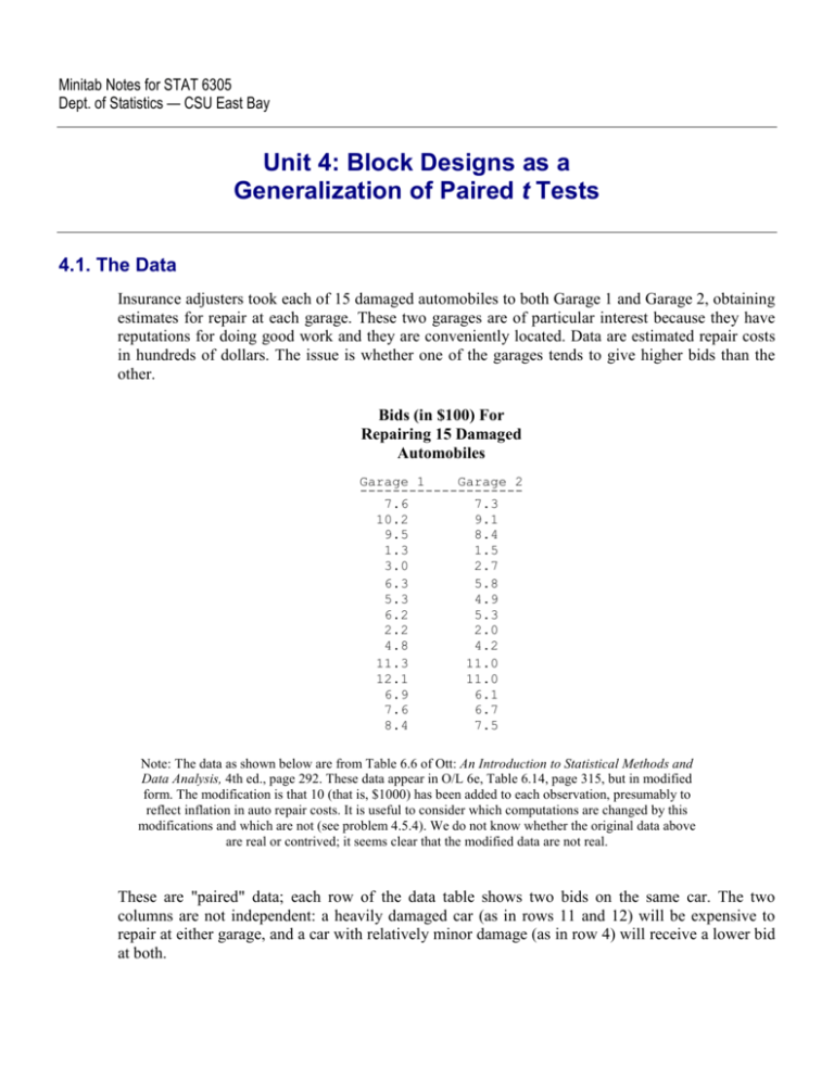
Insurance adjusters took each of 15 damaged automobiles to both Garage 1 and Garage 2, obtaining
estimates for repair at each garage. These two garages are of particular interest because they have
reputations for doing good work and they are conveniently located. Data are estimated repair costs
in hundreds of dollars. The issue is whether one of the garages tends to give higher bids than the
other.
Bids (in $100) For
Repairing 15 Damaged
Automobiles
Garage 1
Garage 2
-------------------7.6
7.3
10.2
9.1
9.5
8.4
1.3
1.5
3.0
2.7
6.3
5.8
5.3
4.9
6.2
5.3
2.2
2.0
4.8
4.2
11.3
11.0
12.1
11.0
6.9
6.1
7.6
6.7
8.4
7.5
Note: The data as shown below are from Table 6.6 of Ott: An Introduction to Statistical Methods and
Data Analysis, 4th ed., page 292. These data appear in O/L 6e, Table 6.14, page 315, but in modified
form. The modification is that 10 (that is, $1000) has been added to each observation, presumably to
reflect inflation in auto repair costs. It is useful to consider which computations are changed by this
modifications and which are not (see problem 4.5.4). We do not know whether the original data above
are real or contrived; it seems clear that the modified data are not real.
These are "paired" data; each row of the data table shows two bids on the same car. The two
columns are not independent: a heavily damaged car (as in rows 11 and 12) will be expensive to
repair at either garage, and a car with relatively minor damage (as in row 4) will receive a lower bid
at both.
Minitab Notes for STAT 6305
Unit 4-2
Problems
4.1.1. This problem deals with preparation of the data for exploration and analysis.
(a) Label c1 and c2 of a Minitab worksheet as Gar1 and Gar 2, respectively. Then cut
these data from Word or your browser and paste them into c1 and c2. (When pasting, put
the cursor in the first row of c1; use spaces as delimiters).
(b) Anticipating our work in the next section, put the differences in bids into c3, labeled Diff.
CALC > Calculator, results in c3, expression c1 - c2
MTB > let c3 = c1 - c2
(c) Print the results to the Session Window and verify that they are correct. Your output
should be similar to that shown below, except that the display shown here has been edited
into three panels for more compact display.
DATA > Display Data
MTB > print c1 - c3
ROW
Gar1
Gar2
Diff
ROW
Gar1
Gar2
Diff
ROW
Gar1
Gar2
Diff
1
2
3
4
5
7.6
10.2
9.5
1.3
3.0
7.3
9.1
8.4
1.5
2.7
0.3
1.1
1.1
-0.2
0.3
6
7
8
9
10
6.3
5.3
6.2
2.2
4.8
5.8
4.9
5.3
2.0
4.2
0.5
0.4
0.9
0.2
0.6
11
12
13
14
15
11.3
12.1
6.9
7.6
8.4
11.0
11.0
6.1
6.7
7.5
0.3
1.1
0.8
0.9
0.9
4.1.2. Suppose that you have 30 randomly chosen damaged cars available. How could this
experiment have been designed in order to produce data that are not paired? Rewrite the first
sentence of this section (above the data) to indicate the experimental procedure you have in mind to
produce two independent columns of data. Which design, paired or independent, do you think is
best for the purpose at hand, and why?
4.1.3. Return now to the original paired-data experiment. It can be viewed as a two-factor
experiment. One factor is Garage and the other is Car. In Units 1 and 2 we dealt with fixed factors,
the levels of which are determined to be of particular interest to the experimenters. For example. the
three levels of type of hot dogs in Unit 2 were Beef, Meat, and Poultry. In Unit 3 we dealt with a
random factor, in which the levels were four randomly chosen batches. The individual batches are
of interest only insofar as they may reflect random batch-to-batch variability. In the current
experiment, one of the factors is fixed and the other is random. Which is the fixed factor, which is
the random factor, and why?
4.2. Descriptive Techniques
Separate dotplots for the two repair shops mainly show the high variability among the 15 cars as to
the amount of damage to be repaired. But a comparison of the two dotplots shows no important
difference between the garages. This graphical comparison is ineffective partly because we do not
know which dot in one plot compares to which dot in the other; the paired nature of the data is
obscured.
Minitab Notes for STAT 6305
Unit 4-3
> Dotplot > Multiple Y's simple, select 'Gar1' and 'Gar2' (GPRO plot)
gstd
dotp c1 c2;
same.Dotplot
GRAPH
MTB >
MTB >
SUBC>
.
.
.
. .
.. . :
.
. .
.
.
---+---------+---------+---------+---------+---------+---Gar1
. .
.
.
. . . . . ..
.
.
:
---+---------+---------+---------+---------+---------+---Gar2
2.0
4.0
6.0
8.0
10.0
12.0
However, if we look at a dotplot of the differences (below), we see that all but one are positive.
Thus Garage 1 tends to give higher bids than Garage 2. From this dotplot we can also see that, on
average for our small sample of cars, bids from Garage 1 are about $60 higher than those from
Garage 2. If the two garages have equivalent bidding rules, it is difficult to imagine that such a large
difference resulted just because of random error.
GRAPH > Dotplot > One Y Simple (GPRO plot)
MTB > gstd
MTB > dotp c3
Dotplot
.
.
.
.
.
:
.
.
.
.
:
:
+---------+---------+---------+---------+---------+-------Diff
-0.25
0.00
0.25
0.50
0.75
1.00
Problems
4.2.1. It was claimed above that we should expect the bids by the two garages to be associated. (For
example, a heavily damaged car will get a high bid at both garages.) Make a scatterplot of Gar1
vs. Gar2 and describe what you see. (Where do the points lie relative to the line Gar 1 = Gar2?)
Note that the syntax for a scatterplot in gpro mode requires an asterisk (*) between the column
numbers. (Menu path and commands shown; results not shown.)
Graph > Plot
MTB gpro # (if needed)
MTB plot c1 * c2
4.2.2. Reproduce the two dotplots on the same scale as shown above. Make a printout and connect
each dot for Garage 1 with the corresponding dot (same damaged car) for Garage 2. (The plot at the
top of the next page shows similar information; it was made using a procedure intended for another
purpose, so the label Means should read Bid.)
Minitab Notes for STAT 6305
Unit 4-4
Plot Showing the Paired Nature of the Data
Auto
1
2
3
4
5
6
7
8
9
10
11
12
13
14
15
12
10
Mean
8
6
4
2
0
1
2
Gar
4.3. Paired t Test
Assuming that the data are approximately normally distributed, an appropriate test to confirm what
we saw in the dotplot of the differences is a paired t test. In Minitab, this can be performed as a onesample t test of the null hypothesis that the population of differences has zero mean. We conclude
that the difference between garages is highly significant, as indicated by the P-value < 0.00005.
STAT > Basic > 1-sample t, test mean = 0
MTB > ttest 0 c3
TEST OF MU = 0.000 VS MU N.E. 0.000
N
15
Diff
MEAN
0.613
STDEV
0.394
SE MEAN
0.102
T
6.02
P VALUE
0.0000
Recent releases of Minitab have a paired procedure that finds the differences and performs the
above test on them with a single command (or menu box). The two columns used must be of equal
length. Compare the printout below with the one just above.
STAT > Basic > Paired-t
MTB > Paired c1 c2
Paired T-Test and CI: Gar1, Gar2
Paired T for Gar1 - Gar2
Gar1
Gar2
Difference
N
15
15
15
Mean
6.84667
6.23333
0.613333
StDev
3.20399
2.94125
0.394365
SE Mean
0.82727
0.75943
0.101825
95% CI for mean difference: (0.394941, 0.831725)
T-Test of mean difference = 0 (vs not = 0): T-Value = 6.02
P-Value = 0.000
Minitab Notes for STAT 6305
Unit 4-5
It is crucial to take the paired nature of the data into account. If we had incorrectly analyzed these
data using a two-sample t test, we would have failed to detect the significant effect; note the 0.589
P-value below. (This is the computational equivalent of the incorrect and futile graphical comparison of the separate dotplots for the two garages that we made in Section 4.2.)
INCORRECT PROCEDURE
STAT > Basic > 2-sample t, different columns, assume equal variances
MTB > twos c1 c2;
SUBC> pool.
Two-Sample T-Test and CI: Gar1, Gar2
Two-sample T for Gar1 vs Gar2
Gar1
Gar2
N
15
15
Mean
6.85
6.23
StDev
3.20
2.94
SE Mean
0.83
0.76
Difference = mu (Gar1) - mu (Gar2)
Estimate for difference: 0.613333
95% CI for difference: (-1.687000, 2.913667)
T-Test of difference = 0 (vs not =): T-Value = 0.55
Both use Pooled StDev = 3.0754
P-Value = 0.589
DF = 28
Problems
4.3.1. Looking at the dotplot of differences one may legitimately wonder whether they are normally
distributed. Perform one of the three formal tests of normality available in the menu path
STAT > Basic > Normality. Give the P-value and say what it indicates. Also try the normal
probability plot in the menu path GRAPH > Normal probability plot. What device does the
latter plot use to help you judge whether the data are normal?
Note: The null hypothesis of normality is not rejected. But even if this hypothesis had been
rejected at the borderline, many statisticians would say that the conclusion from the t test is still
valid. The criteria for using the t test are that (i) the sample size is moderately large, (ii) there is
no obvious skewness, and (iii) there are no outliers. The Central Limit Theorem suggests that
the sample mean would be nearly normally distributed, even if the original data were not.
These criteria indicate that the t statistic has nearly a t-distribution.
4.3.2. If one chose to do a nonparametric test, either a sign test (STAT > Nonparametrics >
1-Sample Sign; command stest 0 c3) or a Wilcoxon signed-rank test (STAT ð
Nonparametrics > 1-Sample Wilcoxon; command wtest 0 c3) would be appropriate.
Remember that, for these tests, the null hypothesis is that the population of differences has zero
median. Perform both tests, give P-values, and interpret the results.
4.3.3. In Problem 3.1.4 you were asked to consider redesigning this experiment so that the data are
in two independent groups. Could data collected in this way be correctly analyzed according to the
two-sample t procedure shown at the end of this section? Explain briefly.
Minitab Notes for STAT 6305
Unit 4-6
4.4. Stacked Data
An important goal of this unit is to show that a randomized block design is a generalization of the
paired t test shown above. However, we need to put the data into stacked format before we can
continue. [Instead of the last subcommand you could use the set command with data (1:2)15.]
MTB > name c11 'Bid' c12 'Garage'
MTB > stack c1 c2 c11;
SUBC> subs c12.
But there is one more step in order for the stacked data to fully represent the structure of the
experiment. We need to identify which car produced which bids. This requires another column
labeled Car. (The results are shown after the problems for this section.)
MTB >
MTB >
DATA>
DATA>
name c13 'Car'
set c13
2(1:15)
end
Now we have Bids in c11, subscripts (1 and 2) for Garages in c12, and subscripts (1 through 15) for
Cars in c13. Below is a printout of the stacked data. Study it carefully to make sure that you understand how all of the information in the columns Gar1 and Gar2 has been re-expressed in the columns
Bid, Garage, and Car. (For your convenience, columns Gar1 and Gar2 are shown again.)
STACKED FORMAT
----------------------------ROW
Bid
Garage
Car
UNSTACKED FORMAT
-------------------ROW
Gar1
Gar2
1
2
3
4
5
7.6
10.2
9.5
1.3
3.0
1
1
1
1
1
1
2
3
4
5
1
2
3
4
5
7.6
10.2
9.5
1.3
3.0
7.3
9.1
8.4
1.5
2.7
6
7
8
9
10
6.3
5.3
6.2
2.2
4.8
1
1
1
1
1
6
7
8
9
10
6
7
8
9
10
6.3
5.3
6.2
2.2
4.8
5.8
4.9
5.3
2.0
4.2
11
12
13
14
15
11.3
12.1
6.9
7.6
8.4
1
1
1
1
1
11
12
13
14
15
11
12
13
14
15
11.3
12.1
6.9
7.6
8.4
11.0
11.0
6.1
6.7
7.5
16
17
18
19
20
7.3
9.1
8.4
1.5
2.7
2
2
2
2
2
1
2
3
4
5
21
22
23
24
25
5.8
4.9
5.3
2.0
4.2
2
2
2
2
2
6
7
8
9
10
26
27
28
29
30
11.0
11.0
6.1
6.7
7.5
2
2
2
2
2
11
12
13
14
15
Minitab Notes for STAT 6305
Unit 4-7
In stacked format each row gives full information on how a particular bid arose—its amount, which
garage, and which car. The order in which these self-sufficient rows are recorded in the worksheet
is not important for an analysis of variance. For example, as long as each row stays intact, it is not
necessary for all of the bids for Garage 1 to appear first, nor for the Cars to be listed in any particular order. However, if the data were collected in a particular known order (one would hope based on
randomization), then the actual order of collection should be reflected in the order of the rows of the
stacked format in the worksheet. (In each format, locate the data for the first four five cars.)
Problems
4.4.1. Which format would you choose if you were presenting data in a report, stacked or
unstacked? Give reasons briefly.
4.4.2. How could the data table at the very beginning of this unit be modified to make it clearer to
the reader that the data are paired and that each row shows the results for a particular car?
4.4.3. In conducting an experiment such as this one, damaged cars would be sampled and then each
car would be taken to the two garages to get bids for repair. Perhaps the toss of a coin would decide
whether a particular car was taken to Garage 1 or Garage 2 first. Which format, stacked or unstacked,
would be natural for recording the results of this experiment as data collection progresses?
4.5. Block Design
The randomized block design, explained in Ott/Longnecker (Sec. 15.3), is a generalization of the
two-sided paired t test that is able to handle more than two treatments. The word block should be
considered as a generalization of the word pair. When paired data are treated according to a block
design, the conclusion should be the same as for the paired t test. We use Minitab's balanced
ANOVA procedure to analyze the data as a block design.
STAT > ANOVA > Balanced, Response: Bid,
Model: Garage Car, Random: Car, Storage: Residuals
MTB > anova c11 = c12 c13;
SUBC> random c13;
SUBC> restrict;
SUBC> resids c14.
ANOVA: Bid versus Garage, Car
Factor
Garage
Car
Type
fixed
random
Factor
Garage
Car
Values
1, 2
1, 2,
Levels
2
15
3,
4,
5,
6,
7,
8,
9, 10, 11, 12, 13, 14, 15
Analysis of Variance for Bid
Source
Garage
Car
Error
Total
DF
1
14
14
29
S = 0.278858
SS
2.821
263.742
1.089
267.652
MS
2.821
18.839
0.078
R-Sq = 99.59%
F
36.28
242.26
P
0.000
0.000
R-Sq(adj) = 99.16%
Minitab Notes for STAT 6305
Unit 4-8
Notes on Minitab's anova procedure:
•
The notation for the model (in the "Model" box for the menu, or after the equal sign (=) for the
command) is shorthand for the model:
Yij = µ + αi + Bj + eij,
where i = 1, 2; j = 1, ..., 15; Σαi = 0; Bj iid N(0, σB2); and eij iid N(0, σ2). A grand mean µ
and an error term must be present in every ANOVA model, and so there is no need for these
terms to appear in the syntax. What we must mention is c12 (Garage) and c13 (Car), together
with the column of measurements c11 (Bid).
•
We take Garage to be a fixed effect (Greek letter α) because the two garages are of specific
interest. Perhaps they are the garages most conveniently located to an insurance company that
routinely seeks bids. The restriction that the α's sum to 0 is expressed in the subcommand
restrict.
•
We take Car to be a random effect (Latin letter B) because the 15 cars are chosen at random.
Minitab requires random effects to be declared using the subcommand random.
•
With a design as simple as the current one, it happens that no damage would have resulted in the
output if the commands random and restrict had been omitted. However, we shall soon
see models for which these specifications are crucial, and it is a good idea to start now to
include all of the specifications needed to make the model correct.
•
The residuals subcommand is used to store the residuals from the model in empty column
c14. (When using the subcommand residuals be careful to use an empty column because this
subcommand will overwrite data without warning. With menus, Minitab automatically selects
an empty column for the residuals, but it may not be especially conveniently located in the
worksheet.)
The F-ratio for testing the Garage effect is F = 2.8213 / 0.0778 = 36.3. The corresponding P-value,
printed as 0.000 indicates a value smaller than 0.0005. Clearly, the difference between the garages
is highly significant.
This F test is equivalent to the paired t test performed above. F = 36.3 = (6.02)2 is the square of the
t-statistic for the paired t test. (Depending on the release of Minitab and the procedure used, the
P-value may be written as 0.0000, meaning less than 0.00005, or 0.000, but even if expressed to
different numbers of decimal places, the value represented are actually the same.)
The Car effect ("block effect") can be tested with the statistic F = 18.8387 / 0.0778 = 242.26; it is
very highly significant. Of course, this is no surprise. We used Cars as blocks precisely because we
anticipated large differences from car to car.
The reason for introducing the blocking factor into an experimental design is the suspicion that it
will be significant, thus helping to explain variability that would otherwise have wound up inflating
MS(Error), making the F-ratio for the "main" effect small, and possibly leading to a Type II error.
(See Problem 4.5.4 for an illustration.) If Blocks are not significant, it may be a signal that a block
design should not have been used.
In performing any ANOVA you should always generate the residuals and look at them graphically,
usually starting with a boxplot and a normal probability plot. The symmetry of the normal
probability plot results from the fact that there are only two observations per Car and thus each car
gives two residuals equal in absolute value and opposite in sign.
Minitab Notes for STAT 6305
Unit 4-9
The normal probability plot of the residuals is shown below. It is not precisely linear, but the
departure from normal is not extreme. (Various tests of normality have P-values around 0.1. The
result of the Anderson-Darling test is shown as part of the plot below.)
Such a plot can be made from Graphs option in menu box for the balanced ANOVA. or, after
storing residuals, or by using the menu path shown below . Without some practice, the precision of
the high resolution plot (and the way it treats repeated values) can lead to over-interpretation of
small deviations from linearity. It is a good idea for beginners to include "error bands" in their high
resolution plots. (See the graph on the next page.
GRAPH > Probability plot > Single, select residuals
Normal Probability Plot of Residuals
Normal - 95% CI
ANOVA for Block Design
99
Mean
StDev
N
AD
P-Value
95
90
-5.18104E-17
0.1938
30
0.614
0.100
Percent
80
70
60
50
40
30
20
10
5
1
-0.75
-0.50
-0.25
0.00
RESI1
0.25
0.50
Problems
4.5.1. Suppose we want to use the fixed significance level 1% for testing whether there is a
difference between the two garages. Find the critical values for both the paired t test and the F test
of the block procedure. Show that the square of the critical values of t is the critical value of F.
Note: Critical values for a given significance level can be obtained by using the invcdf
command; or by selecting CALC ð Probability distributions ð t (or F), inverse
from menus. The inverse cumulative distribution function gives the cut-off value
that has a designated probability below; adjust appropriately to get the critical values for each
test. The t-distribution has 14 degrees of freedom; there is 1 degree of freedom in the numerator
and there are 14 degrees of freedom in the denominator of the F-distribution.
cumulative
4.5.2. Use Minitab's general linear model procedure (STAT > ANOVA > GLM) to get mainly the same
output as at the beginning of this section. Notice that the standardized residuals for one of the cars
are (barely) greater than 2 in absolute value and hence the observations for that car are noted as
Minitab Notes for STAT 6305
Unit 4-10
"unusual." Which car? Make a boxplot of the residuals (or standardized residuals). What outliers, if
any, are indicated?
4.5.3. Earlier in this unit we looked at nonparametric alternatives to the one-sample t test. There
are also nonparametric alternatives for analyzing a block design. Perhaps the best known of them
is the Friedman test (menu path STAT ð Nonparametrics ð Friedman or command
friedman c11 c12 c13). Do the Friedman test for the present data and interpret the result.
4.5.4. Read the footnote to the data table in section 4.1. Add 10 to each observation shown in the
table and repeat the ANOVA of section 4.5 for the modified data. Comment on which results
changed and which did not. Would a linear transformation of the data affect the F-statistic?
4.5.5. In this problem we ask you to perform two INCORRECT procedures so that you will
understand the consequences of ignoring or misunderstanding the block structure of an
experimental design. What result do you obtain if you analyze the data (as given in section 4.1):
• As a one-way ANOVA, ignoring Cars?
• As a one-way ANOVA, ignoring Garages?
Why is each of these analyses incorrect? Which one corresponds to the incorrect two-sample t test
done at the end of Section 4.3?
Finally, compare the values of MS(Error) for the correct analysis as a block design and for the
incorrect analysis ignoring Cars, and comment. In this comparison, what two sums of squares in the
correct ANOVA table sum to SS(Error) in the incorrect one? Can the correct ANOVA table be
constructed from information in the two incorrect tables?
4.5.6. For some years, the "Taster's Choice" column was a regular feature in the Wednesday Food
Section of the San Francisco Chronicle. The column of December 17, 2003 reported results when
five professional tasters rated four brands of creamy horseradish (a common condiment for prime
rib of beef), declaring Mezzetta as the "winner." The taster's scores are shown below. Treat Tasters
as random blocks (analogous to Cars in the example of this unit) and Brands of horseradish as the
fixed main effect (analogous of Garages). Each score is out of a total of 20 points. According to the
appropriate ANOVA, are there any statistically significant differences among brands? (Because
there are now more than two observations per block a paired t test is no longer an option. In a
subsequent unit we take a more careful look at such block designs.)
BRAND
---------------------------------------TASTER
Mezzetta
Sosnick
Beaver
Tulelake
-----------------------------------------------------Carroll
16
13
16
3
Halperin
19
10
9
13
Hatfield
18
14
12
16
Katzl
16
16
14
16
Passot
16
16
16
9
Minitab Notes for Statistics 6350 by Bruce E. Trumbo, Department of Statistics, CSU East Bay, Hayward CA, 94542,
Email: bruce.trumbo@csueastbay.edu. Comments and corrections welcome. Copyright © 1991, 2010 by Bruce E.
Trumbo. All rights reserved. These notes are intended for use by students at California State University, East Bay.
Please contact the author for permission to use elsewhere. Preparation partially supported by NSF grant USE-9150433.
Modified: 1/10