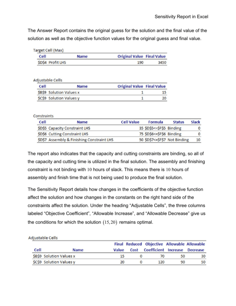
Sensitivity Report in Excel
The Answer Report contains the original guess for the solution and the final value of the
solution as well as the objective function values for the original guess and final value.
The report also indicates that the capacity and cutting constraints are binding, so all of
the capacity and cutting time is utilized in the final solution. The assembly and finishing
constraint is not binding with 10 hours of slack. This means there is 10 hours of
assembly and finish time that is not being used to produce the final solution.
The Sensitivity Report details how changes in the coefficients of the objective function
affect the solution and how changes in the constants on the right hand side of the
constraints affect the solution. Under the heading “Adjustable Cells”, the three columns
labeled “Objective Coefficient”, “Allowable Increase”, and “Allowable Decrease” give us
the conditions for which the solution 15, 20  remains optimal.
Sensitivity Report in Excel
For instance, if the coefficient on x is raised to 70  50  120 , or decreased to 70  30  40
40, the optimal production plan is to produce 15 frame bags and 20 panniers. Similarly, if
the coefficient on y is raised to 120  90  210 , or decreased to 120  50  70 , the optimal
production plan remains unchanged.
In each case, we can calculate the range of values that the coefficient can take on by
subtracting the allowable decrease from the coefficient or adding the allowable increase
to the coefficient.
In terms of the application, this means that if the profit per frame bag varies between 40
and 120 or the profit per pannier varies between 70 and 210, the optimal production plan
is to produce 15 frame bags and 20 panniers per week. These values match the values
we discovered earlier in the section using the graph of the feasible region.
The second part of the Sensitivity Report examines how changes to the right hand side
of any constraint affects the optimal solution. A change to the constant on the right hand
side of a constraint changes the size of the feasible region. Increasing the right hand
side of any constraint with positive coefficients shifts the border matching the constraint
up. Decreasing the right hand side of any constraint with positive coefficients shifts the
border matching the constraints down. The shadow price indicates how the objective
function will change when the constant on the right hand side is changed.
In the table, the shadow price for the capacity constraint is 45. This indicates that if the
capacity is increased by 1 (from 35 to 36), the corresponding profit at the optimal
solution will increase by $45. Similarly, if the capacity is decreased by 1 (from 35 to 34),
the profit at the optimal solution will decrease by $45. In both cases, since the size of
the feasible region changes, the optimal solution changes to a new value.
Sensitivity Report in Excel
These changes are valid over a range of changes indicated by the values in the
“Allowable Increase” and “Allowable Decrease” columns. As long as the right hand side
stays within 35  10  25 to 35  4  39 , the shadow price is valid.
The same reasoning applies to the other binding constraint in the linear programming
problem. If the amount of time for cutting increases/ decreases by 1 hour in a range of
values from 75  20  55 hours to 75  30  105 hours, the profit will increase/decrease by
$25.
The sensitivity analysis for a nonbinding constraint, like the assembly and finishing
constraint, is different. At the optimal solution, changes to the right hand side do not
affect the profit as long as the right hand side is not decreased too much. This means
that the shadow price is $0. The only way this would change is if the number of hours
for assembly and finishing is dropped to 50 hours. At this point, there is no longer any
slack at the optimal solution and the constraint becomes binding.
This fact is evident in the report under the “Allowable Decrease” column.
For the assembly and finishing constraint, the shadow price of $0 is applicable for a
decrease of 10 hours from 60 hours or 50 hours. The “Allowable Increase” for this
constraint is show as 1E+30. This is Excel’s way of showing infinity. This means that the
right hand side can be increased any amount without changing the shadow price. This
should make sense since increasing the right hand side (adding more hours for
assembly and finishing) simply adds more unutilized time to the constraint and will not
change the feasible region. As expected, Excel’s Sensitivity Report mirrors the
conclusions we drew from analyzing the constants in the constraints graphically.
Sensitivity Report in Excel
Excel can also be used to find and analyze the solution to a standard minimization
problem.
Example 1
Analyze the Sensitivity Report for a Standard
Minimization Problem
In Sections 4.2 and 4.4, we solved the minimization problem
Minimize C  100Q1  125Q2
subject to
Q1  Q2  10, 000
Q2  0.25Q1
Q2  Q1
Q1  0, Q2  0
where C is the cost of contracting Q1 barrels of American ale from
contract brewery 1 and Q2 barrels of America ale from contract brewery
2.
Use Excel to solve and analyze the associated standard minimization
problem
Minimize C  100Q1  125Q2
subject to
Q1  Q2  10, 000
 0.25Q1  Q2  0
Q1  Q2  0
Q1  0, Q2  0
Solution Follow the steps earlier (with appropriate modifications) to
create the worksheet below.
Sensitivity Report in Excel
Be careful to use the SUMPRODUCT function correctly in cells D4
through D7.
The Solver Parameters are as follows:
Also make sure you set the Solver Options properly. If you do not set
the options properly, the Sensitivity Report will not look like the one
presented earlier.
The worksheet below shows the final solution.
Sensitivity Report in Excel
According to the worksheet, 8000 barrels should be contracted from
brewery 1 and 2000 barrels from brewery 2. This results in a minimum
cost of $1,050,000. Notice that the slack in the second constraint is
-4.5E-13. This is approximately zero and nothing to be concerned about.
By examining the objective coefficients, we can determine the range of
values over which  Q1 , Q2    8000, 2000  remains optimal.
If the cost per barrel at brewery 1 is as high as 100  25  125 dollars or
as low as 100  131.25  31.25 dollars and we hold the cost per barrel at
brewery 2 at $125, this solution remains optimal. The cost per barrel
cannot be negative so realistically the cost per barrel can be between
$0 and $125.
If the cost per barrel at brewery 2 is greater than 125  25  100 dollars
and the cost per barrel is held constant at $100, the solution is still
optimal. The number 1E+30 under allowable increase indicates the
coefficient can be increased without bound.
Sensitivity Report in Excel
Now let’s look at the other table in the Sensitivity Report.
The first constraint requires that the breweries supply at least 10,000
barrels and is binding. The shadow price of $105 is valid for a
production requirement as low as 10, 000  10, 000  0 and infinitely high.
The shadow price of $105 indicates that if the production requirement is
increased by one barrel within this range, the cost will increase by $105.
The shadow price for the second constraint indicates how the cost will
change if the right hand side of 0.25Q1  Q2  0 is increased by one
barrel. Since this inequality is equivalent to Q2  0  0.25Q1 , increasing
the constant by 1 unit is the same as changing the requirement that the
number of barrels from brewery 2 be at least one quarter the number of
barrels from brewery 1 to a requirement that the number of barrels from
brewery 2 must be at least one more than one quarter of the number of
barrels from brewery 1. With this change in the requirement, the cost
will increase by $20. This cost increase is valid for constants on the right
side from -2500 to 3750.
Sensitivity Report in Excel
The third constraint is not binding. As long as the constant on the right
hand side of Q1  Q2  0 is less than 6000, changing the constant by one
barrel does not change the cost.