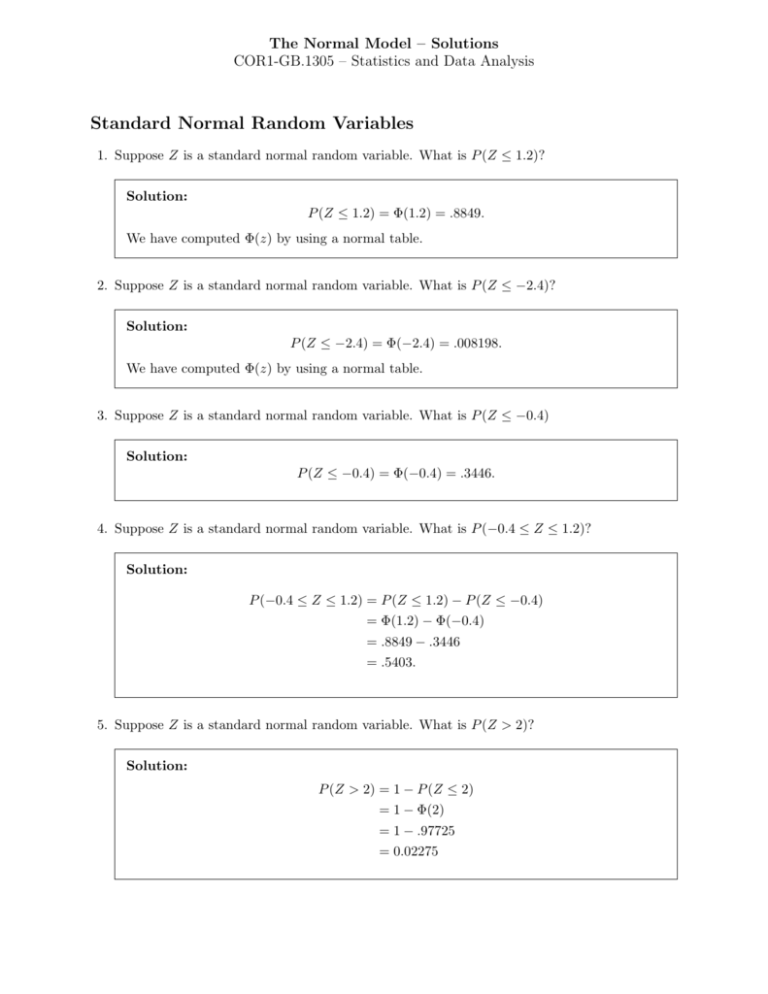
The Normal Model – Solutions
COR1-GB.1305 – Statistics and Data Analysis
Standard Normal Random Variables
1. Suppose Z is a standard normal random variable. What is P (Z ≤ 1.2)?
Solution:
P (Z ≤ 1.2) = Φ(1.2) = .8849.
We have computed Φ(z) by using a normal table.
2. Suppose Z is a standard normal random variable. What is P (Z ≤ −2.4)?
Solution:
P (Z ≤ −2.4) = Φ(−2.4) = .008198.
We have computed Φ(z) by using a normal table.
3. Suppose Z is a standard normal random variable. What is P (Z ≤ −0.4)
Solution:
P (Z ≤ −0.4) = Φ(−0.4) = .3446.
4. Suppose Z is a standard normal random variable. What is P (−0.4 ≤ Z ≤ 1.2)?
Solution:
P (−0.4 ≤ Z ≤ 1.2) = P (Z ≤ 1.2) − P (Z ≤ −0.4)
= Φ(1.2) − Φ(−0.4)
= .8849 − .3446
= .5403.
5. Suppose Z is a standard normal random variable. What is P (Z > 2)?
Solution:
P (Z > 2) = 1 − P (Z ≤ 2)
= 1 − Φ(2)
= 1 − .97725
= 0.02275
Normal Cumulative Distribution Function (CDF)
6. The dressed weights of Excelsior Chickens are approximately normally distributed with mean
3.20 pounds and standard deviation 0.40 pound. About what proportion of the chickens have
dressed weights greater than 3.60 pounds?
Solution: Let X be the weight of a typical chicken in pounds; this is normally distributed
with mean µ = 3.20 and standard deviation σ = 0.40. The proportion of chickens with
dressed weights greater than 3.60 is equal to the probability that X is greater than 3.60
pounds.
Define Z = (X − µ)/σ, a standard normal random variable. Then,
X − µ
3.60 − µ >
σ
σ
3.60 − 3.20 =P Z>
0.40
= P(Z > 1)
P(X > 3.60) = P
= 1 − P(Z ≤ 1)
= 1 − Φ(1)
= 1 − .8413
= .1587.
Page 2
7. Suppose that an automobile muffler is designed so that its lifetime (in months) is approximately
normally distributed with mean 26 months and standard deviation 4 months. The manufacturer
has decided to use a marketing strategy in which the muffler is covered by warranty for 18
months. Approximately what proportion of the mufflers will fail before the warranty expires?
Solution: Let X be the lifetime of a typical muffler in months; this is normally distributed
with mean µ = 26 and standard deviation σ = 4. The muffler will fail before the warranty
expires if and only if X < 18. Thus, the proportion of the mufflers that fail before the
warranty expires is equal to the probability that X is less than 18. Define Z = (X − µ)/σ,
a standard normal random variable. Then,
X − µ
18 − 26 <
σ
4
= P (Z < −2)
P(X < 18) = P
= Φ(−2)
= .02275.
8. Suppose that the daily demand for change (meaning coins) in a particular store is approximately
normally distributed with mean $800.00 and standard deviation $60.00. What is the probability
that, on any particular day, the demand for change will be below $600?
Solution: Let X be the demain for change on a particular day (in dollars); this is a normal
random variable with mean µ = 800 and standard deviation σ = 60. Now
X −µ
600 − 800
P(X < 600) = P
<
= Φ(−3.3) = .0004834.
σ
60
Page 3
Inverse Normal CDF
9. Suppose that the daily demand for change (meaning coins) in a particular store is approximately
normally distributed with mean $800.00 and standard deviation $60.00. Find the amount M
of change to keep on hand if one wishes, with certainty 99%, to have enough change. That is,
find M so that P(X ≤ M ) = 0.99.
Solution: We have
.99 = P (X ≤ M ) = P
X −µ
M − 800
≤
σ
60
=Φ
M − 800
60
.
Thus,
M − 800
= Φ−1 (.99).
60
Consulting the normal inverse CDF table, we see that Φ(2.3263) = .99 and We take
Φ−1 (.99) = 2.3263, so that
M = 800 + 60 × 2.3263 = 939.578.
10. Suppose that Z is a standard normal random variable. Find the value w so that P(|Z| ≤ w) =
0.60.
Solution: The problem is asking for w such that P(−w ≤ Z ≤ w) = 0.60. We can look
up this value directly, in the fourth column, getting w = .8416.
For an alternative solution, note that
P(Z < −w) + P(−w ≤ Z ≤ w) + P (Z > w) = 1.
Also, P(Z < −w) = P(Z > w) (draw a picture if this is not obvious to you). In this case,
we must have that P(Z < −w) = 0.20. Therefore, P(Z < w) = 0.80.
Now, Φ(w) = 0.80. The normal CDF table tells us that Φ(0.8416) = 0.80; we take w =
0.8416.
11. A machine that dispenses corn flakes into packages provides amounts that are approximately
normally distributed with mean weight 20 ounces and standard deviation 0.6 ounce. Suppose
that the weights and measures law under which you must operate allows you to have only 5%
of your packages under the weight stated on the package. What weight should you print on
the package?
Page 4
Solution: Let X be the weight in ounces of a typical package; this is approximately normally distributed with mean µ = 20 and standard deviation σ = 0.6. We seek a printed
weight, w, such that P (X < w) = .05. Define Z = (X − µ)/σ, a standard normal random
variable. We have the following relation:
X −µ
w − 20
w − 20
w − 20
.05 = P(X < w) = P
=P Z<
=Φ
.
<
σ
0.6
0.6
0.6
Thus,
w − 20
= Φ−1 (.05).
0.6
With a normal table, we compute Φ(−1.6449) = 0.05. Finally,
w − 20
= −1.6449,
0.6
so w = 20 − 0.6 × 1.6449 = 19.01306. We would probably round this to 19 and print “19
ounces” on the box.
Page 5