Representing Conditional Independence Using Decision Trees
Jiang Su and Harry Zhang
Faculty of Computer Science
University of New Brunswick, NB, Canada, E3B 5A3
hzhang@unb.ca
Abstract
While the representation of decision trees is fully expressive theoretically, it has been observed that traditional decision trees has the replication problem. This
problem makes decision trees to be large and learnable
only when sufficient training data are available. In this
paper, we present a new representation model, conditional independence trees (CITrees), to tackle the replication problem from probability perspective. We propose a novel algorithm for learning CITrees. Our experiments show that CITrees outperform naive Bayes (Langley, Iba, & Thomas 1992), C4.5 (Quinlan 1993), TAN
(Friedman, Geiger, & Goldszmidt 1997), and AODE
(Webb, Boughton, & Wang 2005) significantly in classification accuracy.
Introduction
In decision tree learning algorithms, a decision tree is induced from a set of labeled training examples represented
by a set of attribute values and a class label. We denote a
set of attributes by a bold-face upper-case letter, for example, A = (A1 , A2 , · · · , An ), and an assignment of values
to each attribute in an attribute set by a corresponding boldface lower-case letter, for example, a. We use C to denote
the class variable and c to denote its value. Thus, a training
example E = (a, c), where a = (a1 , a2 , · · · , an ), and ai is
the value of attribute Ai .
While decision trees perform quite well in classification,
the representation structure of traditional decision trees suffers from the replication problem (Oliver 1993; Pagallo &
Haussler 1990). Namely, we are forced to represent disjunctive concepts in different branches, which leads to duplication of subtrees. This problem causes decision trees to be
large and learnable only when sufficient training data are
available. Let us see the following example.
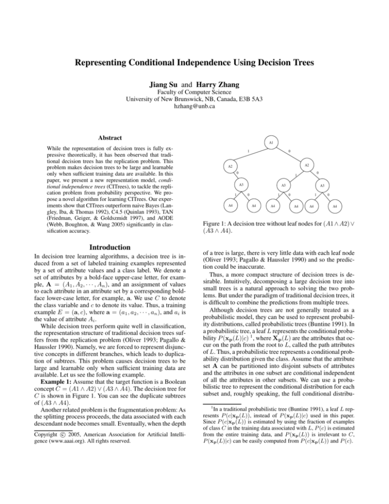
Example 1: Assume that the target function is a Boolean
concept C = (A1 ∧ A2) ∨ (A3 ∧ A4). The decision tree for
C is shown in Figure 1. You can see the duplicate subtrees
of (A3 ∧ A4).
Another related problem is the fragmentation problem: As
the splitting process proceeds, the data associated with each
descendant node becomes small. Eventually, when the depth
c 2005, American Association for Artificial IntelliCopyright gence (www.aaai.org). All rights reserved.
A1
1
0
A2
A2
0
A3
1
A4
0
1
A3
0
1
A4
A4
A3
0
1
A4
A4
0
A4
Figure 1: A decision tree without leaf nodes for (A1 ∧ A2) ∨
(A3 ∧ A4).
of a tree is large, there is very little data with each leaf node
(Oliver 1993; Pagallo & Haussler 1990) and so the prediction could be inaccurate.
Thus, a more compact structure of decision trees is desirable. Intuitively, decomposing a large decision tree into
small trees is a natural approach to solving the two problems. But under the paradigm of traditional decision trees, it
is difficult to combine the predictions from multiple trees.
Although decision trees are not generally treated as a
probabilistic model, they can be used to represent probability distributions, called probabilistic trees (Buntine 1991). In
a probabilistic tree, a leaf L represents the conditional probability P (xp (L)|c) 1 , where Xp (L) are the attributes that occur on the path from the root to L, called the path attributes
of L. Thus, a probabilistic tree represents a conditional probability distribution given the class. Assume that the attribute
set A can be partitioned into disjoint subsets of attributes
and the attributes in one subset are conditional independent
of all the attributes in other subsets. We can use a probabilistic tree to represent the conditional distribution for each
subset and, roughly speaking, the full conditional distribu1
In a traditional probabilistic tree (Buntine 1991), a leaf L represents P (c|xp (L)), instead of P (xp (L)|c) used in this paper.
Since P (c|xp (L)) is estimated by using the fraction of examples
of class C in the training data associated with L, P (c) is estimated
from the entire training data, and P (xp (L)) is irrelevant to C,
P (xp (L)|c) can be easily computed from P (c|xp (L)) and P (c).
tion P (A|C) is equal to the product of conditional probability distributions of all trees. Notice that P (A|C) and the
prior probability P (C) determine a unique classifier.
It is easy to decompose the decision tree for Example 1
into two probabilistic trees corresponding to two concepts
(A1 ∧ A2) and (A3 ∧ A4), respectively, shown in Figure 2.
Notice that all the probabilities are estimated from the truth
table, in which each possible assignment of truth values to
A1 , A2 , A3 , and A4 occurs exactly once. Figure 2 represents
the conditional independence that P (A1 , A2 , A3 , A4 |C) =
P (A1 , A2 |C)P (A3 , A4 |C) (Strictly, that is not true.). It is
easy to verify that Figure 2 represents the target concept C =
(A1 ∧ A2) ∨ (A3 ∧ A4).
P( C=1)=7/16
P( C=0)=9/16
T1
T2
A1
A3
1
0
1
0
A4
A2
A2
1
......
1
p( A1 =1, A2 =1| C =1)=1
p( A1 =1, A2 =1| C =0)=0
0
p( A1 =0, A2 =1| C =1)=1/7
p( A1 =0, A2 =1| C =0)=1/3
0
......
0
......
......
0
1
p( A1 =1, A2 =0| C =1)=1/7
p( A1 =1, A2 =0| C =0)=1/3
A4
1
p( A 1 =0, A2 =0| C =1)=1/7
p( A1 =0, A2 =0| C =0)=1/3
Figure 2: Two probabilistic trees representing (A1 ∧ A2) ∨
(A3 ∧ A4), in which the probabilities in T2 are similar to
that in T1 .
Figure 2 shows us that a compact decision tree presentation can be achieved by representing conditional independence in probabilistic trees. This is the key idea of this paper.
Related Work
Although decision trees performs well in classification,
their replication problem and fragmentation problem are
also well known (Oliver 1993; Pagallo & Haussler 1990).
Those two problems have been attacked from two major
approaches: constructing compound attributes (Oliver 1993;
Pagallo & Haussler 1990), and extending the tree structure
of decision trees to the more complex graph structure, such
as decision graphs (Kohavi 1994). However, no clear solution has emerged under the traditional decision tree paradigm.
It has also been observed that traditional decision tree algorithms, such as C4.5 (Quinlan 1993), produce poor probability estimates(Provost, Fawcett, & Kohavi 1998). A substantial amount of work has been done recently on learning
decision trees with accurate probability estimates (Provost &
Domingos 2003). Although, theoretically, decision trees can
represent any probability distribution, those that yield accurate probabilities tend to be large because of the replication
problem, and the probability estimates could still be poor because of the fragmentation problem. A more compact representation could be an effective solution for this problem.
Although decision trees are well-known as a decision
boundary-based classifier, each leaf of a tree can represent a
conditional probability distribution. One way to extend decision trees toward a probabilistic model is to deploy a local
probability model on leaves of a decision tree (Smyth, Gray,
& Fayyad 1996). Friedman and Goldszmidt (1996) propose
to use decision trees to represent the local distributions in
Bayesian networks, in which only the conditional probability distribution of a single attribute is represented. Recently,
Zhang and Su (2004) propose to use a decision tree to represent conditional independence. They present a type of probabilistic trees, in which, given the path attributes, all other
attributes on a leaf are independent. Their model, however,
is not a general model that can represent any conditional independence. Jaeger (2004) propose a model probabilistic
decision graphs that is based on ordered binary decision diagrams.
In this paper, we present a novel decision tree representation model, conditional independence trees (CITrees).
Our basic idea is to iteratively explore and represent conditional attribute independencies at each step in constructing
a decision tree, and thus decompose a traditional decision
(sub)tree into smaller (sub)trees.
Representing Conditional Independence under
Decision Tree Paradigm
The key feature of decision trees is the iterative and nested
decomposition. The instance space is iteratively partitioned
into subspaces in a decision tree. More precisely, each internal node N corresponds to a subspace defined by the values of the path attributes Xp (N ). It is natural to explore
the conditional independencies among attributes in the subspace. Here the conditioning variables are Xp (N ) and C.
Indeed, some attribute independencies do not exist in the entire instance space, but do exist in some subspaces. This type
of conditional attribute independencies are called contextspecific independence (Boutilier et al. 1996), differentiating
it from the global conditional independence that is conditioned only by C. The structure of decision trees from top
to bottom provides a natural structure for exploring and representing various context-specific independence among attributes in various granularities from coarse to fine.
As discussed in the first section, a leaf L in a probabilistic
tree represents the conditional probability P (xp (L)|c). Let
us denote all the attributes not in Xp (L) by Xl (L), called
non-path attributes. If there is a representation of the conditional probability distribution over the non-path attributes
at each leaf L, denoted by P (xl (L)|xp (L), c), then each
leaf represents a full conditional probability over all the attributes, conditioned by C, as shown in Equation 1. Thus,
a probabilistic tree represents a full conditional distribution
P (A|C).
P (a|c) = P (xl (L)|xp (L), c)P (xp (L)|c).
(1)
Moreover, the subtree with root N represents a conditional
distribution P (Xl (N )|xp (N ), c). In the recursive process
of learning a decision tree, if Xl (N ) can be partitioned into
disjoint and conditional independent subsets Al1 (N ), · · ·,
Alk (N ), we can construct k probabilistic (sub)trees, each of
which represents P (Ali |xp (N ), c), i = 1, · · ·, k, and their
product represents P (Xl (N )|xp (N ), c). Thus, a traditional
probabilistic (sub)tree can be represented by a set of smaller
trees.
Definition 1 Given two attributes Ai and Aj , and a set of
attributes Θij , Ai and Aj are said to be conditionally independent given Θij , if
P (Ai , Aj |Θij , C) = P (Ai |Θij , C)P (Aj |Θij , C).
(2)
Definition 2 Given two sets of attributes U and Θ, and Θ ∩
U = Φ (the empty set), a subset UI is called a conditional
independence set given Θ, or simply CI set, if
1. for any attribute Aj ∈
/ UI , Aj is conditionally independent from any attribute Ai ∈ UI given Θ;
2. UI is the minimum subset satisfying property 1.
Assuming that {UI1 , · · ·, UIk } is a partition of CI sets of
U given Θ, we have
P (U |Θ, C) =
k
Y
(3)
P (UIi |Θ, C).
i=1
Our idea is that, at each step of constructing a probabilistic
tree, we detect conditional attribute dependencies by discovering CI sets. We then build a tree for each CI set by choosing one attribute as the root, and repeat this process for each
of its branches until certain criteria have been met. We use a
rectangle to contain a set of trees, each of which corresponds
to a CI set. A conditional independent tree, or simply CITree, is defined formally as follows.
Definition 3 1. A probabilistic tree (without any rectangle)
is a CITree.
2. A rectangle containing a set of probabilistic trees is a CITree.
3. If T1 , · · ·, Tk are CITrees, then a tree consisting of a root
and subtrees T1 , · · ·, Tk is a CITree.
Example 2: Figure 3 shows a CITree, in which the rectangle containing two subtrees T2 and T3 represents the following context-specific independence.
P (A2 , A3 |A1 = 1, c) = P (A2 |A1 = 1, c)P (A3 |A1 = 1, c).
A1
T1
0
1
A2
T2
A2
0
A3
...
...
A3
1
...
1. If T is a probabilistic tree with root A (a CITree
without rectangle), its conditional probability P (T ) =
P (A|Xp (A), C).
2. If T is represented by a rectangle containing independent
sub-CITrees T1 , · · ·, Tk ,
P (T ) =
k
Y
P (Ti ).
(4)
i=1
3. If T is a single (sub)CITree with root A = {a1 , · · · , ak }
and subtrees Ts (ai ) corresponding to A = ai , i =
1, · · · , k,
P (T ) = P (Ts (ai )), when A = ai .
(5)
A CITree provides, essentially, a more compact representation for the full conditional distribution, given C, than a
probabilistic tree. Combined with P (C), it also determines
a classifier.
Bayesian networks (Pearl 1988) are a well-known probabilistic model. Generally speaking, a Bayesian network represents attribute independencies in the entire instance space,
that is, global independence. It is not natural to use Bayesian
networks to represent various context-specific independencies in different granularities. For example, assume that
Ak+2 depends on Ak+1 only when Ai = ai , i = 1, · · · , k.
To represent this fact in a Bayesian network, Ak+2 should
have k + 1 parents. In a CITree, this dependency is represented by only one path.
Another drawback of Bayesian networks is that it is intractable to learn the optimal structure of a Bayesian network from data. Thus, in practice, imposing restrictions on
the structures of Bayesian networks, such as tree-augmented
naive Bayes (TAN) (Friedman, Geiger, & Goldszmidt 1997),
in which each attribute is allowed to have a parent only from
other attributes, has been accepted. In contrast, CITrees have
a tree structure, substantially simpler than a graph structure.
It could be expected that learning a good CITree is easier
than learning a good Bayesian network.
Notice the difference between CITrees and the work of
Boutilier et al. (1996). In their work, context-specific independence is explored within the framework of Bayesian
networks, not iteratively from various granularities as CITrees do. Moreover, a decision tree is used only to represent
the local distribution of a single attribute.
1
0
0
T3
A3
Definition 4 Assume that T is a (sub)CITree on attribute set
A = (A1 , A2 , · · · , An ), the conditional distribution P (T )
represented by T is defined as follows.
0
...
0
1
...
...
1
...
1
...
Figure 3: CITree for Example 2.
The conditional probability distribution represented by a
CITree T is defined formally as follows.
Learning Conditional Independence Trees
To learn a CITree from data, the first issue is to explore conditional attribute independencies. More concretely, it is how
to partition an attribute set into CI sets. We use conditional
mutual information, defined in Equation 6, to detect the dependency between two attributes.
IP (X; Y |Z) =
X
x,y,z
P (x, y, z)log
P (x, y|z)
,
P (x|z)P (y|z)
(6)
where x, y, and z are the values of variables X, Y , and Z
respectively.
In practice, we focus on strong attribute dependencies,
while ignoring weak attribute dependencies. We define a
threshold based on the Minimum Description Length (MDL)
principle to filter out weak dependencies, defined in Equation 7.
δ(Ai , Aj ) =
log|D|
× |Tij |,
2|D|
(7)
where |D| is the size of the local training data, and |Tij | =
|Ai | × |Aj |. Roughly speaking, |Tij | represents the size increase for representing the dependency between Ai and Aj
in a CITree. In our implementation, Ai and Aj are put into
a CI set, if and only if I(Ai ; Aj |C) > δ(Ai , Aj ). δ(Ai , Aj )
is essentially a threshold. In Example 1, A1 , A2 , A3 and
A4 can be grouped into two CI sets {A1 , A2 } and {A3 , A4 }
using an appropriate threshold. Thus, Figure 2 is learnable.
After exploring the conditional attribute independencies
in the local training data, we get CI set(s). For each CI set
UI , a (sub)CITree is built. We first introduce a few definitions that are used in choosing the root attribute in our algorithm.
Definition 5 Given a CI set UI and an attribute Ai ∈ UI ,
the most influent attribute of Ai , denoted by Ainf
i , is defined
as follows.
Ainf
= arg
i
max
Aj ∈UI ,j6=i
(8)
I(Ai , Aj |C).
Definition 6 In a CI set UI , an attribute Ai is called a composite attribute, if it satisfies the following equation.
I(C; Ai |Ainf
) > I(C; Ai ) + δ(Ai , A iinf ).
i
(9)
Intuitively, a composite attribute is an attribute that is
more useful in discriminating the class variable combined
with other attribute.
Definition 7 The discriminating score of attribute Ai , denoted by ψ(Ai ), is defined as follows:
ψ(Ai ) = max{I(C; Ai ), I(C; Ai |Ainf
)},
i
(10)
where I(C, Ai ) is the mutual information between C and
Ai , defined in Equation 11.
X
P (C, Ai )
I(C; Ai ) =
P (C, Ai )log
C,Ai
P (C)P (Ai )
.
(11)
Ai
Definition 10 The influence score of attribute Ai , denoted
by ω(Ai ), is defined as follows.
X
(12)
(I(C; Aj |Ai )−I(C; Aj )−δ(Ai , Aj )). (13)
ω(Ai ) =
Aj ∈Ψ(Ai )
Definition 10 reflects the influence of attribute Ai on other
attributes in forming composite attributes.
Now we are ready to talk about choosing the root attribute.
One straightforward way is to consider each attribute individually and choose the attribute based on Equation 11. In
fact, C4.5 adopts this strategy. A more sophisticated strategy is to consider the combination of attributes. Our strategy is to consider the most discriminating attribute and its
most influent attribute. An interesting observation from our
experiments is that choosing which one first from the most
discriminating attribute and its most influent attribute is crucial, if the most discriminating attribute is composite. Thus,
we define the influence score for an attribute to distinguish
them. The process for choosing the root attribute consists of
two steps: computing the most discriminating attribute Adis
based on the discriminating scores of attributes, and then
choose one from Adis and its most influent attribute Ainf
dis
based on their influence scores. Notice that we use a threshold in Equation 9 and 13 to handle the overfitting issue.
Building a CItree is also a greedy and recursive process,
similar to building a decision tree. At each step, after discovering CI sets, choose the “best” attribute for each CI set
as the root of the (sub)tree, split the local training data into
disjoint subsets corresponding to the values of the root attribute, and then recur this process for each subset until all
attributes have been used.
Algorithm CITrees(S, U)
Input : a set S of labeled examples, and a set U of attributes.
Output : a CITree.
1. If U is empty Return an empty tree.
2. Identify a partition {UI1 , · · · , UIk } of CI sets of U.
3. For each CI set UIi
4.
Create an empty tree Ti .
5.
Choose the attribute Adis using Equation 12.
6.
In Definition 7, we take the combination of two attributes
into account. In reality, it often happens that the combination of attributes is more useful in discriminating the class
variable C.
Definition 8 The most discriminating attribute for the class
variable C, denoted by Adis , is defined as follows.
Adis = arg max ψ(Ai ).
Definition 9 Given an attribute Ai , the influenced set of Ai ,
denoted by Ψ(Ai ), consists of all the attributes that are composite attributes with Ai as the most influent attribute.
If Ai is composite and ω(Ainf
dis ) > ω(Adis )
7.
Then Aroot = Ainf
dis
8.
elseAroot = Adis
9.
Make Aroot the root of tree Ti .
10.
For all values a of Aroot
11.
Ta = CITrees(Sa , A − {Aroot }).
12.
Add Ta as a child of Aroot .
13. If (k = 1) Return T1 .
14. Else Return a rectangle containing T1 , · · ·, Tk .
Experiments
We conducted experiments to compare our algorithm CITrees with C4.5 (Quinlan 1993), naive Bayes (Langley, Iba,
& Thomas 1992), TAN (Friedman, Geiger, & Goldszmidt
1997), and AODE (averaged one-dependence estimators)
(Webb, Boughton, & Wang 2005). AODE is a newly developed model which demonstrates a remarkable performance.
We implemented CITrees within the Weka framework (Witten & Frank 2000), and used the implementations of naive
Bayes, C4.5(J48), TAN, and AODE in Weka. We chose the
33 UCI data sets from Weka. In our experiment, the accuracy of an algorithm on each data set has been obtained via
10 runs of 10-fold stratified cross validation. Numeric attributes are discretized using ten-bin discretization implemented in Weka. Missing values are also processed using
the mechanism in Weka. In our implementation, we used the
Laplace estimation to avoid the zero-frequency problem. We
conducted a two-tailed t-test with a 95% confidence level to
compare each pair of algorithms on each data set.
Table 1 shows the accuracies of the algorithms on each
data set, and the average accuracy and standard deviation on
all data sets are summarized at the bottom of the table. Table
2 shows the results of the two-tailed t-test, in which each entry w/t/l means that the algorithm in the corresponding row
wins in w data sets, ties in t data sets, and loses in l data sets,
compared to the algorithm in the corresponding column. The
detailed results displayed in Table 1 and Table 2 show that
the performance of CITrees is overall the best among the algorithms compared in this paper. Now, we summarize the
highlights briefly as follows:
1. CITrees perform better than C4.5 (7 wins and 1 loss),
TAN (7 wins and 1 loss), and AODE (9 wins and 3 losses).
2. CITrees significantly outperform naive Bayes (12 wins
and 0 loss).
3. CITrees achieve the highest average accuracy among all
algorithms.
Figure 4 shows an example of a CITree learned from the
“Vowel” data set. In this example, the CITree algorithm generated a CITree with the “SpeakerNumbers” attribute as the
root, and all other attributes are conditionally independent
given the value of “SpeakerNumbers”. This CITree has only
151 nodes, significantly smaller than the tree of 600 nodes
generated by C4.5. More important, the accuracy of CITree
is 94.35%, significantly higher than C4.5’s 75.57%.
Table 2: Summary of the experimental results.
CITree
NB
AODE
TAN
NB
12-21-0
AODE
9-21-3
1-18-14
TAN
7-25-1
3-19-11
5-24-4
C4.5
7-25-1
8-11-14
11-18-4
10-19-4
Conclusions
In this paper, we present a novel decision tree representation model CITrees. CITrees provide a compact repre-
Speaker
Number
0
Featu
re 0
.........
Featu
re 10
15
..............
Featu
re 0
.........
Featu
re 10
Figure 4: The CITree induced from the “Vowel” data set.
sentation by iteratively exploring and representing contextspecific attribute independencies from various granularities. Roughly speaking, a traditional probabilistic (sub)tree
can be decomposed into smaller CITrees. CITrees can be
viewed as a general probabilistic representation model, just
as Bayesian networks. However, CITrees can efficiently represent context-free independence from various granularities,
whereas Bayesian networks can efficiently represent global
independence. We proposed an algorithm for learning CITrees and conducted experiments to compare it with other
state-of-the-art algorithms.
Since the structure of CITrees is significantly simpler than
the structure of Bayesian networks, we believe that the CITree learning algorithm could be considerably simpler than
Bayesian network learning algorithms. There is thus considerable potential room for improving the CITree learning
algorithm presented in this paper. Another interesting question is: Can CITrees be used as a general inference model
just as Bayesian networks are? This paper only addresses
the classification problem.
References
Boutilier, C.; Friedman, N.; Goldszmidt, M.; and Koller,
D. 1996. Context-specific independence in Bayesian networks. In Proceedings of the 12th Annual Conference on
Uncertainty in AI (UAI), 416–422.
Buntine, W. 1991. Theory refinement on Bayesian networks. In Proceedings of the Seventh Conference on Uncertainty in Artificial Intelligence. Morgan Kaufmann. 52–
60.
Friedman, N., and Goldszmidt, M. 1996. Learning
Bayesian networks with local structure. In Twelfth Conference on Uncertainty in Artificial Intelligence. 252–262.
Friedman, N.; Geiger, D.; and Goldszmidt, M. 1997.
Bayesian network classifiers. Machine Learning 29:131–
163.
Jaeger, M. 2004. Probabilistic decision graphs - combining
verification and AI techniques for probabilistic inference.
Table 1: Experimental results on accuracy.
Dataset
Anneal
Audiology
Autos
Balance
Breast-cancer
Wisconsin-breast
Horse-colic
Credit-rating
German-credit
Pima-diabetes
Glass
Cleveland
Heart-statlog
Hepatitis
Hypothyroid
Ionosphere
Iris
Chess
Labor
Letter
Lymphography
Mushroom
Primary-tumor
Segment
Sick
Sonar
Soybean
Splice
Vehicle
Vote
Vowel
Waveform
Zoo
Mean
NB
94.32 ± 2.23
71.4 ± 6.37
63.67 ± 11.36
91.44 ± 1.3
72.94 ± 7.71
97.3 ± 1.75
79.65 ± 5.9
84.75 ± 3.83
75.93 ± 3.87
75.68 ± 4.85
57.69 ± 10.07
83.58 ± 6.4
83.78 ± 5.41
83.53 ± 10.47
92.79 ± 0.73
90.86 ± 4.33
94.33 ± 6.79
87.79 ± 1.91
95.67 ± 8.28
70.09 ± 0.93
85.97 ± 8.88
95.52 ± 0.78
47.2 ± 6.02
89.03 ± 1.66
96.78 ± 0.91
76.35 ± 9.94
92.2 ± 3.23
95.42 ± 1.14
61.03 ± 3.48
90.21 ± 3.95
66.09 ± 4.78
79.97 ± 1.46
93.98 ± 7.14
82.33 ± 4.78
C4.5
98.65 ± 0.97
77.22 ± 7.69
80.44 ± 8.46
64.14 ± 4.16
75.26 ± 5.04
92.19 ± 3.16
84.77 ± 5.89
85.32 ± 4.42
72.61 ± 3.49
73.89 ± 4.7
58.14 ± 8.48
79.44 ± 6.43
79.78 ± 7.71
81.5 ± 8.24
93.24 ± 0.44
87.47 ± 5.17
96 ± 4.64
99.44 ± 0.37
84.97 ± 14.24
81.31 ± 0.78
78.21 ± 9.74
100 ± 0
41.01 ± 6.59
93.42 ± 1.67
98.16 ± 0.68
71.09 ± 8.4
92.63 ± 2.72
94.17 ± 1.28
70.74 ± 3.62
96.27 ± 2.79
75.57 ± 4.58
72.64 ± 1.81
92.61 ± 7.33
82.49 ± 4.71
Int. J. of Uncertainty, Fuzziness and Knowledge-based Systems 12:19–24.
Kohavi, R. 1994. Bottom-up induction of oblivious readonce decision graphs. In Proceedings of the 5th European
Conference on Machine Learning. Springer. 154–169.
Langley, P.; Iba, W.; and Thomas, K. 1992. An analysis of
Bayesian classifiers. In Proceedings of the Tenth National
Conference of Artificial Intelligence. AAAI Press. 223–
228.
Oliver, J. J. 1993. Decision graphs an extension of decision
trees. In Proceedings of the Fourth International Workshop
on Artificial Intelligence and Statistics.
Pagallo, G., and Haussler, D. 1990. Boolean feature discovery in empirical learning. Machine Learning 5(1):71–
100.
Pearl, J. 1988. Probabilistic reasoning in intelligent systems:networks of plausible inference. Morgan Kauhmann.
Provost, F. J., and Domingos, P. 2003. Tree induction for
probability-based ranking. Machine Learning 52(3):199–
215.
Provost, F.; Fawcett, T.; and Kohavi, R. 1998. The case
TAN
98.34 ± 1.18
72.68 ± 7.02
76.98 ± 9.21
86.22 ± 2.82
70.09 ± 7.68
95.05 ± 2.24
80.55 ± 6.23
84.22 ± 4.41
75.86 ± 3.58
75.09 ± 4.96
58.43 ± 8.86
82.78 ± 6.98
79.37 ± 6.87
82.13 ± 9.17
93.23 ± 0.68
92.23 ± 4.36
91.67 ± 7.18
92.05 ± 1.49
87.67 ± 13.77
83.11 ± 0.75
84.07 ± 8.93
99.99 ± 0.03
46.76 ± 5.92
94.54 ± 1.6
97.61 ± 0.73
73.66 ± 10.04
95.24 ± 2.28
95.39 ± 1.16
73.71 ± 3.48
94.57 ± 3.23
93.1 ± 2.85
80.72 ± 1.78
93.69 ± 7.75
84.26 ± 4.82
AODE
96.83 ± 1.66
71.66 ± 6.42
75.09 ± 10.23
89.78 ± 1.88
72.73 ± 7.01
96.91 ± 1.84
81.26 ± 5.83
85.78 ± 3.75
76.45 ± 3.88
76.57 ± 4.53
61.73 ± 9.69
83.07 ± 7.05
83.63 ± 5.32
83.55 ± 9.73
93.56 ± 0.61
91.74 ± 4.28
94 ± 5.88
91.03 ± 1.66
94.73 ± 8.79
85.54 ± 0.68
85.46 ± 9.32
99.95 ± 0.07
47.87 ± 6.37
92.92 ± 1.4
97.52 ± 0.72
79.91 ± 9.6
93.31 ± 2.85
96.12 ± 1
71.65 ± 3.59
94.52 ± 3.19
89.64 ± 3.06
84.24 ± 1.6
94.66 ± 6.38
85.25 ± 4.54
CITree
99.29 ± 0.87
79.18 ± 7.6
80.84 ± 8.4
91.44 ± 1.29
70.91 ± 7.54
97.2 ± 1.83
80.71 ± 5.82
84.81 ± 4.03
74.58 ± 3.62
75.52 ± 4.71
60.43 ± 8.94
82.38 ± 6.86
81.96 ± 5.73
84.07 ± 9.09
93 ± 0.69
91.97 ± 4.26
94.2 ± 6.47
99.03 ± 0.52
93.4 ± 10.57
87.22 ± 0.72
85.7 ± 8.02
100 ± 0
43.78 ± 6.59
94.52 ± 1.54
97.82 ± 0.83
77.99 ± 9.96
94.08 ± 2.78
94.56 ± 1.46
72.38 ± 3.76
95.52 ± 2.89
94.35 ± 2.5
81.43 ± 1.65
95.75 ± 6
85.75 ± 4.47
against accuracy estimation for comparing induction algorithms. In Proceedings of the Fifteenth International Conference on Machine Learning. Morgan Kaufmann. 445–
453.
Quinlan, J. 1993. C4.5: Programs for Machine Learning.
Morgan Kaufmann: San Mateo, CA.
Smyth, P.; Gray, A.; and Fayyad, U. 1996. Retrofitting
decision tree classifiers using kernel density estimation.
In Proceedings of the Twelfth International Conference on
Machine Learning. Morgan Kaufmann. 506–514.
Webb, G. I.; Boughton, J.; and Wang, Z. 2005. Not so naive
bayes: Aggregating one-dependence estimators. Journal of
Machine Learning 58(1):5–24.
Witten, I. H., and Frank, E. 2000. Data Mining –Practical
Machine Learning Tools and Techniques with Java Implementation. Morgan Kaufmann.
Zhang, H., and Su, J. 2004. Conditional independence
trees. In Proceedings of the 15th European Conference on
Machine Learning. Springer. 513–524.