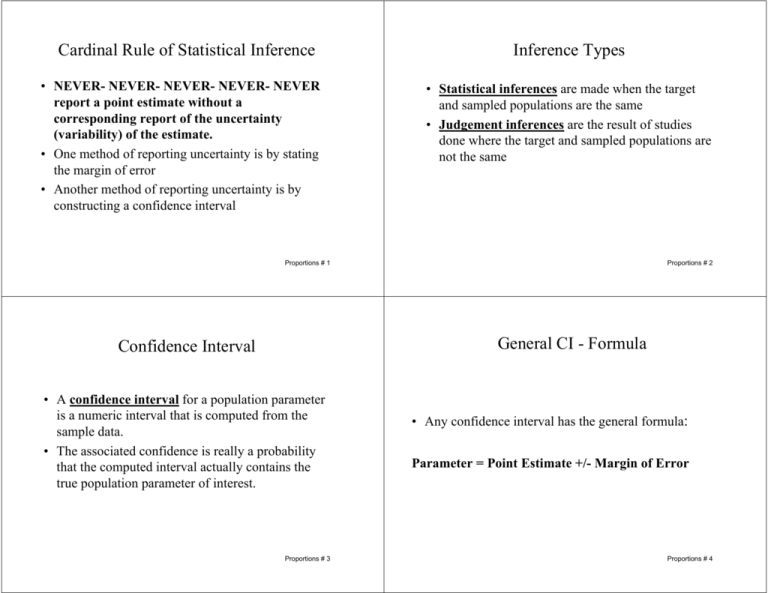
Cardinal Rule of Statistical Inference
• NEVER- NEVER- NEVER- NEVER- NEVER
report a point estimate without a
corresponding report of the uncertainty
(variability) of the estimate.
• One method of reporting uncertainty is by stating
the margin of error
• Another method of reporting uncertainty is by
constructing a confidence interval
Inference Types
• Statistical inferences are made when the target
and sampled populations are the same
• Judgement inferences are the result of studies
done where the target and sampled populations are
not the same
Proportions # 1
Proportions # 2
General CI - Formula
Confidence Interval
• A confidence interval for a population parameter
is a numeric interval that is computed from the
sample data.
• The associated confidence is really a probability
that the computed interval actually contains the
true population parameter of interest.
Proportions # 3
• Any confidence interval has the general formula:
Parameter = Point Estimate +/- Margin of Error
Proportions # 4
Margin of Error (ME)
Endpoints
• The margin of error is the measure of the
variability associated with the point estimate at the
desired level of confidence
• Small margins of error imply a higher precision
than large margins of error
• The higher the desired confidence level, the larger
the margin of error
Proportions # 5
• A confidence interval is made up of two endpoints
which enclose a range of values.
• The lowest value in the computed confidence interval
is called the Lower Endpoint.
• The largest value in the computed confidence interval
is called the Upper Endpoint.
Proportions # 6
Interpretation of Confidence Intervals
Confidence Level
• This is a proportion associated with ANY confidence
interval.
• Most often confidence levels of 0.90, 0.95, 98, and 0.99
are used.
• You might also hear the intervals associated with these
values referred to as 90, 95, 98,and 99 percent
confidence intervals
Proportions # 7
• One popular interpretation is that, “After the
experiment is done the investigator is 95%
(or 90 or 99%) certain (confident) that the
computed interval contains the TRUE
population parameter of interest.”
• We will use this definition for class
purposes.
Proportions # 8
The Point Estimate
Computing the point estimate
• Just as we used the sample mean as the
point estimate for the true population mean
– so we use the sample proportion as the
point estimate for the true population
proportion.
• The sample proportion is denoted as: p̂
• To compute p-hat, use the following
formula:
pˆ =
number of outcomes of interest
n
Proportions # 9
Margin of Error (ME)
Proportions # 10
CI’s for Proportions
To Compute ME for the sample proportion
you use:
Parameter = Point Estimate +/- Margin of Error
ME = z •
( pˆ )(1 − pˆ )
n
Proportions # 11
p = pˆ ± z •
( pˆ )(1 − pˆ )
n
Proportions # 12
Compute the Point Estimate
Example
A political pollster would like to estimate the true
proportion of the population of county residents
that favor a controlled growth ballot issue. A SRS
of 350 county residents found that 230 of them
favored the issue. Use this information to
construct a 95% CI for the true proportion of
residents who favor the issue.
• Another way to think of successes is to view a
“success” as an outcome of interest. In this
example the outcome of interest is “favoring” the
ballot issue
• So the point estimate is:
pˆ =
230
= 0 . 657
350
Proportions # 13
Find the z-value
• There are 4 popular
levels of confidence.
Each one has its own
corresponding z-value
• In this example CL =
95% so the z-value is
1.96
CL
Proportions # 14
Compute the ME - 1
z-value
90%
1.645
95%
1.96
98%
2.33
99%
2.58
Proportions # 15
ME = z •
ME = 1 .96 •
( pˆ )(1 − pˆ )
n
( 0.657 )(1 − 0 .657 )
350
Proportions # 16
Compute the ME - 2
Confidence Interval
• Now put everything together
ME
= 1 . 96 •
( 0 . 657 )( 0 . 343 )
350
= 1 . 96 •
. 000644
Parameter = Point Estimate +/- Margin of Error
p = 0.657 ± 0.0497
= 1 . 96 ( 0 . 0254 )
= 0 . 0497
pl = 0.657 - 0.0497 = 0.607
pu = 0.657 + 0.0497 = 0.707
= (0.607, 0.707)
Proportions # 17
Interpretation of Confidence Intervals
• The English interpretation follows the format
described for interpreting confidence intervals
described in a previous slide
• In this case, we are 95% confident that the true
proportion of county voters in favor of the ballot
issue is between 0.607 and 0.707
• Note that you might also interpret in terms of
percentages
Proportions # 19
Proportions # 18
Sample Size Determination
Population Proportions
• Researchers often want to plan a study to insure that the
uncertainty in the point estimate will not exceed some
specified value.
• Another way to state this is that the investigators would
like to be sure that, at the end of the study, a CI for the
parameter of interest does not exceed some prescribed
width or that the ME doesn’t exceed some specified
value.
Proportions # 20
Sample Size Determination
• The superintendent of a large school district wants to
estimate p, the proportion of first-graders who have
not had their immunization shots. She plans to use a
SRS of first-graders to obtain the estimate and she
wants to be 95% confident that the point estimate p̂ will
be no more than 0.05 units from the true value of p.
Sample Size Determination – The
conservative approach
• In order to obtain a CI at a specified level of
confidence and ME you need to take “n” observations
where:
z2
n=
4E 2
Proportions # 21
Sample Size Determination if you have
an estimate of p
• What do we know?
1) E = 0.05
2) p̂ = 0.10
3) (1 − pˆ ) = 1 - 0.10 = 0.90
4) z comes from the ttable. For a 95% CI the
value of z = 1.96
Proportions # 22
Sample Size Determination if you
have an estimate of p
• Now it’s just plug-n-chug
z2
n =
4E 2
1 . 96 2
=
2
4 (0 . 05 )
= 384 . 2 → 385
•Note that we ALWAYS round up!!
Proportions # 23
Proportions # 24
Capture/Mark/Recapture
The Estimation of
Population Size
• In order to wisely manage the annual elk hunting
season the division of wildlife would like to
estimate the total number of elk in the state.
• In order to determine whether or not to remove a
species from the endangered species list the EPA
wants to estimate the population size of that
species.
• Estimation of the sizes of “hard to census”
populations is often carried out via the method of
“capture/recapture”.
• This is a two-stage method.
• During the first stage a group from the population
of interest is captured and marked in some way.
• After a prescribed time has passed a second sample is
“re”captured and the proportion of marked units in this
group is used to compute a sample proportion.
Proportions # 25
Capture/Mark/Recapture
Proportions # 26
Setting
• The value of the sample proportion is used further to
estimate the true population size.
• The underlying premise is, as usual, that the sample is a
good representation of the population.
• In other words, if my resample contains 10% marked units
then we say that the entire population must contain 10%
marked units.
• This means that the number of units caught and marked at
the first stage must have been about 10% of the entire
population of interest.
Proportions # 27
• A wildlife biologist would like to estimate the
number of black bear living in the western part of
the state. She spends the summer capturing and
marking 82 black bear. The following year she
collects another sample of 95 bear. 6 of these had
been marked. Develop a point estimate and
corresponding 95% CI for the population size of
black bear in the western part of the state.
Proportions # 28
Variables and Values
• Let m be the number of bear in the first sample that
were caught and marked:
m = 82
• Let n be the number of bear in the caught in the
recapture phase:
n = 95
• Let k be the number of marked bear present in the
recaptured sample:
k=6
Step 1A: Compute p̂
k
n
6
=
95
= 0 . 0632
pˆ =
Proportions # 29
Step 1B: Interpret p̂
Proportions # 30
Step 2: Solve For N̂
•We can interpret this statistic as:
The estimated proportion of marked bears in
the entire population of bears
• Since we know the total number of marked
bears - because we put the marks on’em - we
can estimate the total number of bears in the
population
Proportions # 31
pˆ Nˆ = m
m
Nˆ =
pˆ
82
0.0632
= 1298 .3 → 1298
=
Proportions # 32
CI for N
CI for p
•We’ll get a CI for N by using the CI for p
•p is the true proportion of marked elk in the
population.
•We don’t have this value but we have an
estimate of it. Recall that p-hat is 0.0632.
Recall that we can construct the CI of a population
proportion by using the relation:
Parameter = Point Estimate +/- Margin of Error
p = pˆ ± z •
( pˆ )( 1 − pˆ )
n
Proportions # 33
Proportions # 34
CI for p
CI for p
• Here p̂ is the estimated proportion of marked bear.
• n is the number of marked critters in the recaptured sample.
• Since we want to develop a 95% CI, the
appropriate z-value is 1.96
Proportions # 35
p = 0 . 0632 ± 1 . 96
( 0 . 0632 )( 1 − 0 . 0632 )
95
= 0 . 0632 ± 0 . 0489
= ( 0 . 0143 , 0 . 112 )
Proportions # 36
CI for N
CI for N
• Just as we used p̂ to obtain an estimate for N so
we’ll use the interval endpoints to obtain a CI for
N
• Call the upper endpoint: p̂u
• And call the lower endpoint: p̂l
• Now use the endpoints of the CI for p to get the
endpoints for the CI for N
• The upper endpoint is:
m
pˆ l
• And the lower endpoint will be:
m
pˆ u
Proportions # 37
CI for N
Proportions # 38
Interpretation of the CI
• Now use the endpoints of the CI for p to get the
endpoints for the CI for N
82
= 5734 . 3 → 5734
0 . 0143
82
= 732 . 1 → 732
• And the lower endpoint will be:
0 . 112
• The upper endpoint is:
Proportions # 39
• This CI is interpreted like all of the other
confidence intervals we’ve looked at thus far.
• That is: We are 95% confident that the true
number of bears in the population is between 732
and 5734.
• Note that this is a very wide interval and would
probably be of little use!
Proportions # 40
The Estimation of
Population Totals
The Estimation of
Population Totals
• In 2002, the estimated total number of
highway deaths where alcohol was a
contributing factor is: ______________
• The estimated number of practicing
Catholics in Larimer County is: ________
• The estimated number of college
undergraduates who use recreational drugs
is: _________________
• These statistics are computed in three steps
1) Estimate the proportion of the population
with the characteristic of interest
2) Construct a CI for this estimate
3) Use the values computed in steps 1 and 2 to
obtain estimates and limits for the total number of
units in a population that exhibit the characteristic
of interest
Proportions # 41
The Estimation of
Population Totals
Proportions # 42
Step 1A: Compute p̂
In 2004 a survey was commissioned by the
Wyoming state legislature to estimate the number
of its citizens that were living at or below the
poverty line. In a random sample of 504 of its
residents 63 reported a annual income that placed
them at or below the poverty line.
Proportions # 43
pˆ =
63
504
= 0 . 125
Proportions # 44
The Estimation of
Population Totals
Use census estimates for the population
To estimate the total number of persons
living at or below the poverty line we need
to know the total number of people living in
the state during 2004.
This information is usually obtained through
the national census database
In 2004 the estimated population was
506,529
So the estimated total number of persons
living at or below poverty is:
0.125(506,529) = 63,316
Recall that all reported estimates need to
include a report of the uncertainty
Proportions # 45
Proportions # 46
Uncertainty in estimates of
Population Totals
CI for p
To report uncertainty we’ll use the limits of
the CI for the proportion of Wyoming
residents that are living at or below the
poverty line.
For purposes of illustration we’ll use a 90% level
of confidence
p = pˆ ± z •
( pˆ )( 1 − pˆ )
n
= 0 . 125 ± 1 . 645 ⋅
= (0 . 101 , 0 . 149
Proportions # 47
)
(0 . 125 ) ⋅ (1 −
0 . 125
504
Proportions # 48
)
CI for N
Interpret the CI for N
• The estimated number of Wyoming residents
living at or below the poverty line is 63,316
• We are 90% confident that the true number is
between 51,159 and 75,473
• The lower limit for N:
– Nl = 0.101(506,529) = 51,159
• The upper limit for N:
– Nu = 0.149(506,529) = 75,473
Proportions # 49
Proportions # 50