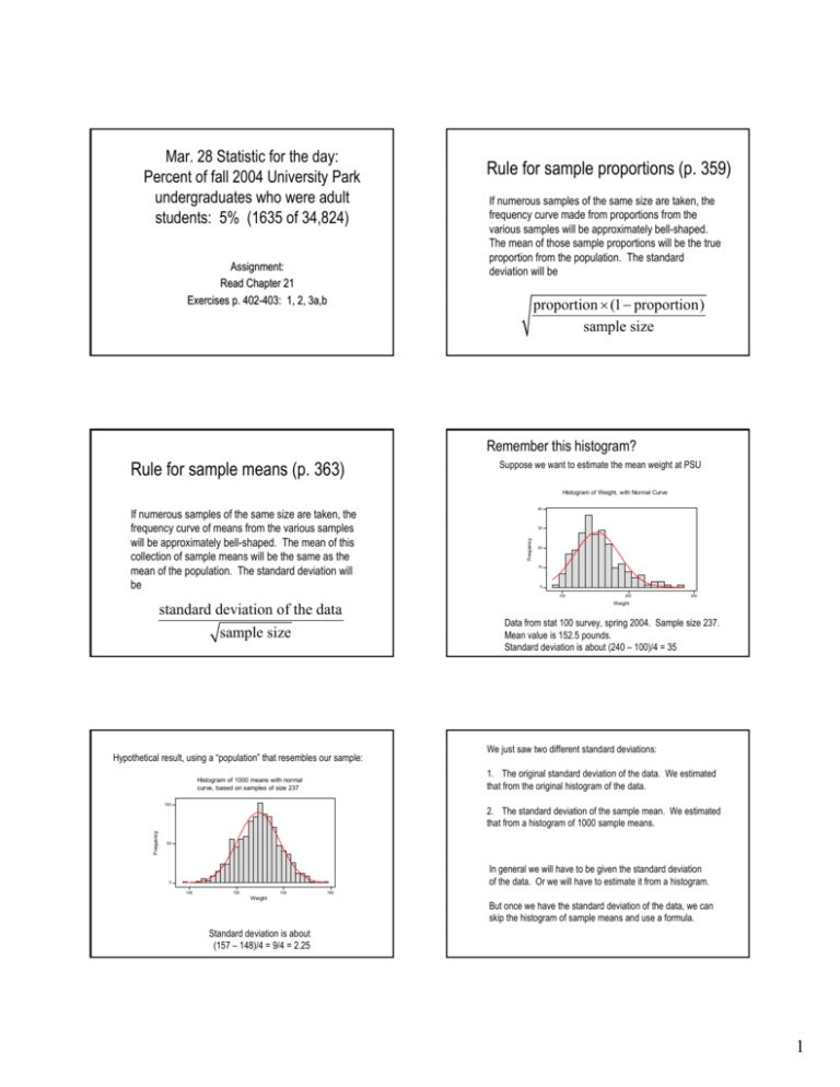
Mar. 28 Statistic for the day:
Percent of fall 2004 University Park
undergraduates who were adult
students: 5% (1635 of 34,824)
Assignment:
Read Chapter 21
Exercises p. 402402-403: 1, 2, 3a,b
Rule for sample proportions (p. 359)
If numerous samples of the same size are taken, the
frequency curve made from proportions from the
various samples will be approximately bell-shaped.
The mean of those sample proportions will be the true
proportion from the population. The standard
deviation will be
proportion × (1 − proportion)
sample size
Remember this histogram?
Rule for sample means (p. 363)
Suppose we want to estimate the mean weight at PSU
Histogram of Weight, with Normal Curve
30
Frequency
If numerous samples of the same size are taken, the
frequency curve of means from the various samples
will be approximately bell-shaped. The mean of this
collection of sample means will be the same as the
mean of the population. The standard deviation will
be
40
20
10
0
100
standard deviation of the data
sample size
Hypothetical result, using a “population” that resembles our sample:
300
Data from stat 100 survey, spring 2004. Sample size 237.
Mean value is 152.5 pounds.
Standard deviation is about (240 – 100)/4 = 35
We just saw two different standard deviations:
1. The original standard deviation of the data. We estimated
that from the original histogram of the data.
Histogram of 1000 means with normal
curve, based on samples of size 237
100
Frequency
200
Weight
2. The standard deviation of the sample mean. We estimated
that from a histogram of 1000 sample means.
50
In general we will have to be given the standard deviation
of the data. Or we will have to estimate it from a histogram.
0
145
150
155
Weight
160
But once we have the standard deviation of the data, we can
skip the histogram of sample means and use a formula.
Standard deviation is about
(157 – 148)/4 = 9/4 = 2.25
1
So in our example of weights:
Formula for estimating the standard deviation of
the sample mean (don’t need histogram)
Suppose we have the standard deviation of the
original sample. Then the standard deviation
of the sample mean is:
Sample size is 237
Hence by our formula:
SEM = SD/square root of sample size
standard deviation of the data
sample size
Standard error of the mean is 35 divided by
the square root of 237: SEM = 35/15.4 = 2.3
Jargon: The standard deviation of the mean is also
called the standard error or the standard error of the mean
and abbreviated SEM or SE Mean.
Using the margin of error of 2 SEMs we really have a
95% confidence interval for the pop mean.
Normal Curve of sample mean.
The standard error is 2.3 and the
bell is centered at 152.5.
8
The standard deviation of the sample is about 35.
Write SD = 35.
So the margin of error of the sample mean is
2×2.3 = 4.6
Report 152.5 ± 4.6 or 147.9 to 157.1
Steps for a 95% confidence interval for a population mean:
1. sample mean: 152.5 (given)
2. sample standard deviation: SD = 35 (given)
3. sample size: 237 (given)
Anatomy of a 95% conf idence interv al
7
6
4. standard error of the mean: SEM = 35/sqrt(237) = 2.3
(you calculate)
5
4
3
5. number of SEMs for 95% confidence: 2 (use p. 157 if needed)
95% in middle
2
1
2 SEM
0
147.9
152.5
sample mean
157.1
True pop mean in here someplace
Example: Estimate mean # of pairs of
jeans owned by a student at PSU
Now put it all together:
6. 95% confidence interval for pop mean: 152.5 ± 2×(2.3)
152.5 ± 4.6 or 147.9 to 157.1
Example: Estimate mean # of pairs of
jeans owned by a student at PSU
50
40
St. Dev. = 5.8 pairs
30
Sample size = 222
20
Mean = 7.8 pairs
SEM =
5.8
= 0.4
222
# of SEMs for 98% confidence: 2.33
Mean = 7.8 pairs
St. Dev. = 5.8 pairs
Sample size = 222
10
98% confidence interval:
0
Frequency
Histogram of Jeans
0
10
20
30
40
Give a 98%
confidence interval.
7.8 ± 2.33×0.4
7.8 ± 0.9, or
6.9 to 8.7
Give a 98%
confidence interval.
Jeans
2
Fibonacci Sequence
Interpretation: We estimate that the population
of Penn State students owns 7.8 pairs of jeans
on average.
98% confidence interval is 6.9 to 8.7 pairs, a
reasonable range of values for the true
(population) mean.
Guess the next numbers in the sequence
1, 1, 2, 3, 5, 8, 13, 21, 34, ...
Called a Fibonacci sequence.
Ratios of pairs after a while equal approximately .618
eg.
8/13 = .615
13/21 = .619
21/34 = .618
width
Daisy
Head
length
If
21 clockwise spirals
34 counterclockwise
width
= .618
length
then the rectangle is called a golden rectangle.
Parthenon in Athens
Villa in Paris by Le Corbusier
3
La Parade
Georges Seurat
St. Jerome
Leonardo
da Vinci
Place de la Concorde
Piet Mondrian
Width to Length ratios for rectangles appearing on beaded
baskets of the Shoshoni
The golden rectangle has become an aesthetic
standard for western civilization.
Width to Length ratio of rectangles in Shoshoni
beaded baskets
0.85
0.75
C1
It appears in many places:
architecture
art
pyramids
business cards
credit cards
0.693 0.662 0.690 0.606 0.570 0.749 0.652 0.628
0.609 0.844 0.654 0.615 0.668 0.601 0.576 0.670
0.606 0.611 0.553 0.633 0.625 0.610 0.600 0.633
0.595
Research question: Do non-western cultures also
incorporate the golden rectangle as an aesthetic standard?
0.65
Golden Rectangle: .618
0.55
Question: Is the golden rectangle (.618) a reasonable
value for the mean of the population of Shoshoni
rectangles?
1.
2.
3.
4.
sample mean: .638
sample standard deviation: SD = .061
sample size: 25
standard error of the mean: SEM = .012
(I calculated it for you.)
How would you create a 95% confidence interval for the
population mean? (We’d like to know whether .618 is in
this interval.)
True or False?
„ To construct a confidence interval for a population
PROPORTION, it is enough to know the sample
proportion and the sample size.
„ To construct a confidence interval for a population
MEAN, it is enough to know the sample mean and the
sample size.
4
Does each of the following tend to make
a confidence interval WIDER or
NARROWER?
„ A larger sample size
„ A larger confidence coefficient
„ A larger standard error of the mean
„ A sample proportion closer to .5
„ A larger sample mean
5