AP Statistics – Ch 4 – More on Two-Variable Data
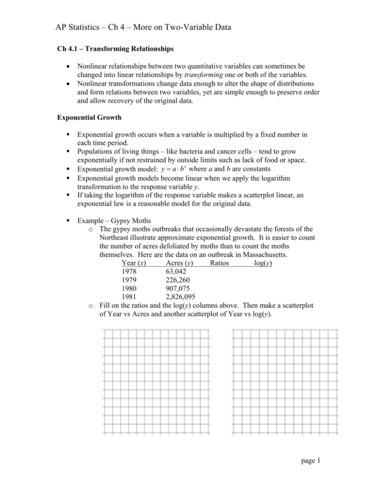
Ch 4.1 – Transforming Relationships
•
•
Nonlinear relationships between two quantitative variables can sometimes be
changed into linear relationships by transforming one or both of the variables.
Nonlinear transformations change data enough to alter the shape of distributions
and form relations between two variables, yet are simple enough to preserve order
and allow recovery of the original data.
Exponential Growth
ƒ
ƒ
ƒ
ƒ
ƒ
ƒ
Exponential growth occurs when a variable is multiplied by a fixed number in
each time period.
Populations of living things – like bacteria and cancer cells – tend to grow
exponentially if not restrained by outside limits such as lack of food or space.
Exponential growth model: y = a ⋅ b x where a and b are constants
Exponential growth models become linear when we apply the logarithm
transformation to the response variable y.
If taking the logarithm of the response variable makes a scatterplot linear, an
exponential law is a reasonable model for the original data.
Example – Gypsy Moths
o The gypsy moths outbreaks that occasionally devastate the forests of the
Northeast illustrate approximate exponential growth. It is easier to count
the number of acres defoliated by moths than to count the moths
themselves. Here are the data on an outbreak in Massachusetts.
Acres (y)
Ratios
log(y)
Year (x)
1978
63,042
1979
226,260
1980
907,075
1981
2,826,095
o Fill on the ratios and the log(y) columns above. Then make a scatterplot
of Year vs Acres and another scatterplot of Year vs log(y).
page 1
AP Statistics – Ch 4 – More on Two-Variable Data
o Find the least squares line fitted to the transformed data.
o Construct and interpret a residual plot for log yˆ on year.
o Perform the inverse transformation to express yˆ as an exponential
equation.
o Use your model to predict the number of acres defoliated in 1982.
page 2
AP Statistics – Ch 4 – More on Two-Variable Data
Power Law Models
ƒ
ƒ
ƒ
ƒ
ƒ
Geometry tells us to expect power laws in some settings. Area goes up with the
square of a dimension and volume goes up with the cube of a linear dimension.
Power Law Model: y = a ⋅ x p
Power law models become linear when we apply the logarithm transformation to
both variables.
If taking the logarithm of both variables makes a scatterplot linear, a power law is
a reasonable model for the original data.
Example – Light Intensity
o The illumination from a light source varies inversely as the square of the
distance from the light source.
o When the distance from a light source is doubled, how does the
illumination change? When the distance from a light source is tripled,
how does the illumination change?
o In physics class, a sensing device at various distances measured the
intensity of a 100-watt light bulb, and the following data were collected.
Distance (meters)
1.0
1.1
1.2
1.3
1.4
1.5
1.6
1.7
1.8
1.9
2.0
Intensity (candelas)
0.2965
0.2522
0.2055
0.1746
0.1534
0.1352
0.1145
0.1024
0.0923
0.0832
0.0734
log(x)
log(y)
o Fill in the log(x) and log(y) columns in the table above.
page 3
AP Statistics – Ch 4 – More on Two-Variable Data
o Make a scatterplot of the Distance vs Intensity and a scatterplot of log(x)
vs log(y).
o Find the least squares line fitted to the transformed data.
o Perform the inverse transformation to express yˆ as a power equation.
o Use your model to predict the light intensity 2.5 meters from the light
source.
page 4
AP Statistics – Ch 4 – More on Two-Variable Data
Ch 4.2 – Cautions about Correlation and Regression
Cautions
ƒ
ƒ
ƒ
ƒ
ƒ
ƒ
Correlation and regression describe only linear relationships.
Correlation r and the least-squares regression line are not resistant (i.e. they are
easily influenced by outliers).
Extrapolation is the use of a regression line for prediction far outside the domain
of values used to obtain the line or curve.
A lurking variable is a variable that is not among the explanatory or response
variables in a study and yet may influence the interpretation of relationships
among those variables.
Correlations based on averages are usually too high when applied to individuals.
That is because, for example, averaging over an entire month smoothes out dayto-day variation.
Example—Hospital Stay
o A study shows that there is a positive correlation between the size of a
hospital (measured by its number of beds x) and the median number of
days y that patients remain in the hospital. Does this mean that you can
shorten a hospital stay by choosing a small hospital? Identify the
explanatory and response variables in this study. Then explain what
lurking variables account for the positive correlation.
The Question of Causation
ƒ
ƒ
Even a very strong association between two variables is not by itself good
evidence that there is a cause-and-effect link between the variables.
A variety of underlying links between variables can explain association. The
dashed line represents an observed association between the variables x and y. The
solid arrow shows the causal relationship.
page 1
AP Statistics – Ch 4 – More on Two-Variable Data
ƒ
ƒ
ƒ
Causation: Changes in x cause changes in y.
Common Response: The observed association between the variables x and y is
explained by a lurking variable z.
Confounding: Both the explanatory variable x and the lurking variable z may
influence the response variable y.
ƒ
Example—Better Readers
o A study of elementary school children, ages 6 to 11 finds a high positive
correlation between shoe size x and score y on a test of reading
comprehension. What explains this correlation?
ƒ
Example—Is Math the Key to Success in College?
o Here is the opening of a newspaper account of a College Board study of
15,941 high school graduates:
o Minority students who take high school algebra and geometry succeed in
college almost the same rates as whites, a new study says. The link
between high school math and college graduation is “almost magical,”
says College Board President Donald Stewart, suggesting “math is the
gatekeeper for success in college.” “These findings,” he says, “justify
serious consideration of a national policy to ensure that all students take
algebra and geometry.”
o What lurking variables might explain the association between taking
several math courses in high school and success in college? Explain why
requiring algebra and geometry may have little effect on who succeeds in
college.
page 2
AP Statistics – Ch 4 – More on Two-Variable Data
Ch 4.3 – Relations in Categorical Data
Marginal Distributions
ƒ
ƒ
ƒ
ƒ
ƒ
ƒ
ƒ
To analyze categorical data, we use the counts or percents of individuals that fall
into various categories.
A two-way table describes two categorical variables.
Values of the row variable label the rows that run across the tables, and the values
of the column variable label the columns that run down the table.
The row totals and column totals give the marginal distributions as percents of the
table total.
Discrepancies in the totals of a two-way table are due to roundoff error.
To describe relationships among categorical variables, calculate appropriate
percents from the counts given.
Example – TV Viewing and Physical Fitness
o Two-way table
Fitness Level
Not Physically Fit
TV Viewing Time Physically Fit
0 hrs
35
137
1-2 hrs
101
629
3-4 hrs
28
222
5 or more hrs
4
44
Total
Total
o Calculate the row and column totals.
o Display the marginal distribution of TV viewing time in terms of percents
by dividing each row total by the table total and converting to a percent.
page 1
AP Statistics – Ch 4 – More on Two-Variable Data
Conditional Distributions
ƒ
ƒ
ƒ
Marginal distributions tell us nothing about the relationship between the variables.
Conditional distributions are when you compare one variable to the different
categories of the other variable.
To find the conditional distribution of the row variable for one specific value of
the column variable, look only at that one column in the table. Find each entry in
the column as a percent of the column total.
ƒ
Example – TV Viewing and Physical Fitness (continued)
o Find the conditional distribution of TV viewing times given that a person
is physically fit.
o Find the conditional distribution of TV viewing times given that a person
is not physically fit.
o Construct a segmented bar graph and describe the differences in TV
viewing time between people that are physically fit and not physically fit.
page 2
AP Statistics – Ch 4 – More on Two-Variable Data
Simpson’s Paradox
ƒ
ƒ
ƒ
Simpson’s Paradox refers to the reversal of the direction of a comparison or an
association when data from several groups are combined to form a single group.
Simpson’s paradox is an example of the effect of lurking variables on an observed
association.
Example – Baseball Paradox
o Most baseball hitters perform differently against right-handed and lefthanded pitching. Consider two players, Joe and Moe, both of whom bat
right handed. The table below records their performance against righthanded and left-handed pitchers.
Player
Joe
Moe
Pitcher
Right
Left
Right
Left
Hits
40
80
120
10
At Bat
100
400
400
100
o Make a two-way table of player (Joe or Moe) versus outcome (hit or no
hit) by summing over both kinds of pitcher.
All Pitchers
Player
Joe
Moe
Total
Hit
Outcome
No Hit
Total
o Find the overall batting average (hits divided by total times at bat) for each
player. Who has the higher batting average?
page 3
AP Statistics – Ch 4 – More on Two-Variable Data
o Make a separate two-way table of player versus outcome for each kind of
pitcher. From these tables, find the batting averages of Joe and Moe
against right-handed pitching. Who does better? Do the same for lefthanded pitching. Who does better?
Right-handed Pitchers
Player
Joe
Moe
Total
Hit
Outcome
No Hit
Total
Outcome
No Hit
Total
Left-handed Pitchers
Player
Joe
Moe
Total
Hit
o The manager doesn’t believe that one player can hit better against both
left-handers and right-handers yet have a lower overall batting average.
Explain in simple language why this happens to Joe and Moe.
page 4