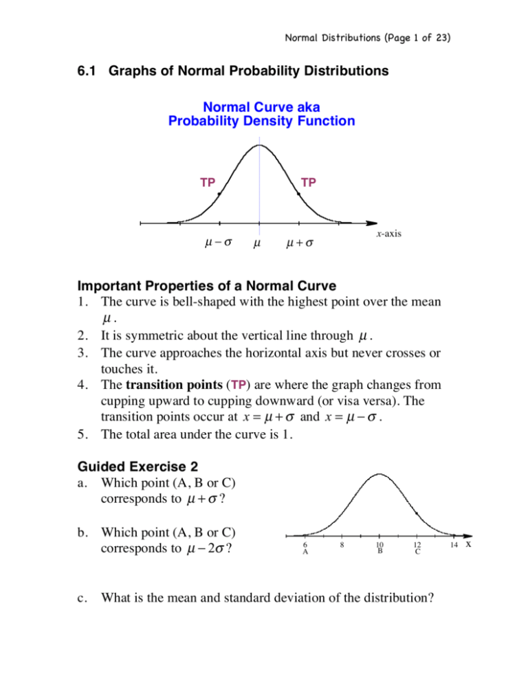
Normal Distributions (Page 1 of 23)
6.1 Graphs of Normal Probability Distributions
Normal Curve aka
Probability
Density
Function
Normal Probability
Distribution
TP
µ !"
TP
x x-axis
µ +!
µ
Important Properties of a Normal Curve
1. The curve is bell-shaped with the highest point over the mean
µ.
2. It is symmetric about the vertical line through µ .
3. The curve approaches the horizontal axis but never crosses or
touches it.
4. The transition points (TP) are where the graph changes from
cupping upward to cupping downward (or visa versa). The
transition points occur at x = µ + ! and x = µ ! " .
5. The total area under the curve is 1.
Guided Exercise1 2
a. Which point (A, B or C)
corresponds to µ + ! ?
b. Which point (A, B or C)
–4
–2
corresponds
to µ ! 2" ?2
c.
4
6
A
8
10
B
12
C
What is the mean and standard deviation of the distribution?
14
x
Normal Distributions (Page 2 of 23)
Example A
The mean affects the location of the curve and the standard
deviation affects the shape (spread) of the curve.
Same Standard Deviation
& Different Means
A
B
Same Mean &
Different Standard Deviations
C
D
Which curve has the
larger mean?
Which curve has the
larger standard
deviation?
Normal Distributions (Page 3 of 23)
Guided Exercise 1
Determine whether each curve
is normal or not. If it is not,
then state why.
Empirical Rule for a Normal Distribution
a. Approximately 68.2% of the data will lie within 1 standard
deviation of the mean.
b. Approximately 95.4% of the data will lie within 2 standard
deviations of the mean.
c. Approximately 99.7% of the data will lie within 3 standard
deviations of the mean.
d. The area under the curve represents the probability and the
total area under the curve is 1.
Empirical Rule
68.2%
0.15%
2.15%
µ ! 3"
13.6%
µ ! 2" µ ! "
13.6%
µ
µ +!
2.15%
µ + 2!
µ + 3!
0.15%
x-axis
Normal Distributions (Page 4 of 23)
Example 1
The playing life of a Sunshine radio is normally distributed with a
mean of 600 hours and a standard deviation of 100 hours.
a. Sketch a normal curve showing the
distribution of the playing life of the
Sunshine radio. Scale and label the axis;
include the transition points.
Use the empirical rule to find the probability
that a randomly selected radio will last
b. between 600 and 700 hours?
c.
between 400 and 500 hours
d. greater than 700 hours?
Normal Distributions (Page 5 of 23)
Guided Exercise 4
The annual wheat yield per acre on a farm is normally distributed
with a mean of 35 bushels and a standard deviation of 8 bushels.
a. Sketch a normal curve and shadein the
area that represents the probability that
an acre will yield between 19 and 35
bushels.
b. Is the shaded area the same as the area between µ ! 2" and
µ ? Use the empirical rule to find the probability that the yield
will be between 19 and 35 bushels per acre?
Control Charts
A control chart for a random variable x that is approximately
normally distributed is a plot of observed x values in time sequence
order. The construction is as follows:
1. Find the mean µ and standard deviation ! of the x
distribution in one of two ways:
(i) Use past data from a period during which the process was
“in control” or
(ii) Use a specified “target” value of µ and ! .
2. Create a graph where the vertical axis represents the x values
and the horizontal axis represents time.
3. Draw a solid horizontal line at height µ and horizontal dashed
control-limit lines at µ ± 2! and µ ± 3! .
4. Plot the variable x on the graph in time sequence order.
Normal Distributions (Page 6 of 23)
Example 2
Susan is director of personnel at Antlers Lodge and hires
many college students every summer. One of the biggest activities
for the lodge staff is to make the rooms ready for the next guest.
Although the rooms are supposed to be ready by 3:30 pm, there are
always some rooms not finished because of high turn over.
Every 15 days Susan has a control chart of the number of
rooms not made up by 3:30 pm each day. From past experience,
Susan knows that the distribution of rooms not made up by 3:30
pm is approximately normal, with µ = 19.3 rooms and ! = 4.7
rooms. For the past 15 days the staff has reported the number of
rooms not made up by 3:30 pm as:
Day 1 2 3 4 5 6 7 8 9 10 11 12 13 14 15
x 11 20 25 23 16 19 8 25 17 20 23 29 18 14 10
a.
Make a control chart for these data. Completely annotate.
Control Chart for the Number
of Rooms Not Made Up by 3:30 PM
µ + 3!
µ + 2!
µ
µ ! 2"
µ ! 3"
b.
Is the housekeeping process out of control? Explain.
Normal Distributions (Page 7 of 23)
Out-of-Control Warning Signals
1. Out-of-Control Signal I: One
point falls beyond the 3! level.
The probability that this is a false
alarm is 0.003.
µ + 3!
µ + 2!
µ
µ + 2!
µ + 3!
2. Out-of-Control Signal II: A run
of 9 consecutive points on one
side of the center line. The
probability that this is a false
alarm is 2 !(0.5)9 = 0.004 .
3. Out-of-Control Signal III: At
least 2 of 3 consecutive points lie
beyond the 2! level on the same
side of the center line. The
probability that this is a false
alarm is 0.002
µ + 3!
µ + 2!
µ
µ + 2!
µ + 3!
µ + 3!
µ + 2!
µ
µ + 2!
µ + 3!
Normal Distributions (Page 8 of 23)
Example 3
Yellowstone Park Medical Services (YPMS) provides emergency
medical care for park visitors. History has shown that the during
the summer the mean number of visitors treated each day is 21.7
with a standard deviation of 4.2. For a 10-day summer period, the
following numbers of people were treated:
Day
1 2 3 4 5 6 7 8 9 10
Number Treated 20 15 12 21 24 28 32 36 35 37
a.
Make a
control chart
and plot the
data on the
chart.
b. Do the data indicate
the number of
visitors treated by
YPMS is in control
or out-of-control?
Explain your
answer in terms of
the three out-ofcontrol signal types.
c.
If you were the park superintendent, do you think YPMS
might need some extra help? Explain.
µ + 3!
µ + 2!
µ
µ ! 2"
µ ! 3"
Normal Distributions (Page 9 of 23)
6.2 Standard Units and
The Standard Normal Distribution
Suppose Tina and Jack are in two different sections of the same
course and they recently took midterms. Tina’s class average was
64 and she got a 74. Jack’s class average 72 and he got an 82.
Who did better?
z-Score or Standardized Score
To standardize test scores we use the z-value or (z-score). The zvalue, or z-score, or standardized score is the number of standard
deviations a data value lies away from the mean. The z-score can
be positive, negative, or zero depending on whether the data value
is above the mean, below the mean, or at the mean, respectively.
For any x-value in a normal
distribution the standardized score, zvalue, or z-score is given by:
Note(s):
1. If x = µ , then z = 0
2. If x > µ , then z > 0
3. If x < µ , then z < 0
z ! score =
x!µ
"
z-score
negative
z-score
positive
x<µ
x>µ
µ
Fact:
Unless otherwise stated, for now on, the average will
mean the arithmetic mean.
x
Normal Distributions (Page 10 of 23)
Example 3
Suppose Tina and Jack are in two different sections of the same
course and they recently took midterms. The distribution of scores
in both classes is normal. Tina’s class average was 64 with a
standard deviation of 3; she earned a 74. Jack’s class average was
72 with a standard deviation of 5; he earned an 82.
a. What was Tina’s z-score? Draw
a distribution for Tina’s class
showing Tina’s score within the
distribution of scores for her
class.
b. What was Jack’s z-score? Draw
a distribution for Jack’s class
showing Jack’s score within the
distribution scores for his class.
c.
Who did better? Why?
Normal Distributions (Page 11 of 23)
Example 4
A pizza parlor chain claims a large pizza has 8 oz of cheese with a
standard deviation of 0.5 oz. An inspector ordered a pizza and
found it only had 6.9 oz of cheese. Franchisee’s can lose their
store if they make pizzas with 3 standard deviations (or more) of
cheese below the mean. Assume the distribution of weights is
normally distributed.
a. Graph the x-distribution.
Label and scale the axis.
b. Find the z-score for x = 6.9
oz of cheese.
c.
Is the franchise in danger of
losing its store? Why?
d. Find the minimum amount of cheese a franchise can put on a
large pizza so it is not in danger of losing its store.
Normal Distributions (Page 12 of 23)
Guided Exercise 6
The times it takes a student to get to class from home is normally
distributed with a mean of 17 minutes and a standard deviation of 3
minutes.
a. One day it took 21 minutes to get to class. How many standard
deviations from the mean is that? Explain the sign.
b. Another day it took 12 minutes to get to class. How many
standard deviations from the mean is that? Explain the sign.
c. On a third day it took 17 minutes to get to class. How many
standard deviations from the mean is that? Explain the sign.
z-Score Formulae
z=
x!µ
"
or
x = z! + µ
Normal Distributions (Page 13 of 23)
Guided Exercise 7
Sam’s z-score on an exam is 1.3.
If the distribution of scores is
normally distributed with a mean
of 480 and a standard deviation
of 70, what is Sam’s raw score.
Draw the distribution.
Standard Normal Distribution / Curve
The standard normal distribution is a normal distribution with
mean µ = 0 and standard deviation ! = 1. The standard normal
curve is the graph of the standard normal distribution.
The Standard Normal Curve
µ = 0, ! = 1
TP
TP
z
Normal Distributions (Page 14 of 23)
The Normal Cumulative Density Function
The area under the normal curve with
mean µ and standard deviation ! on
the interval from a to b represents the
probability that a randomly chosen
value for x lies between a and b. It is
given by the normal cumulative
density function (normalcdf): Access
the DISTR menu (2nd > VARS) and
select 2:normalcdf(lower bound,
upper bound, [ µ , ! ]).
a
b
x
Area = P (a < x < b)
= normalcdf (a,b,[ µ , ! ])
Example 6
Find the probability that z is between -1 and 1.
!3 !2 !1
0
1
2
3
z
Area = P(!1 < z < 1)
= normalcdf (___, ___, ___, ___)
= __________
To show all work and receive full credit
(a) (20-50% of the credit) Sketch the normal curve and shade in
the area in question. Label and scale the axis. Put dots at the
transition points and tick marks on the axis to 3 standard
deviations on each side of the mean.
(b) (50-70% of the credit) Compute the area under the curve,
hence the probability, showing the probability notation, the TI83 function accessed along with its inputs and output. Round
probabilities to 4 decimal places.
Normal Distributions (Page 15 of 23)
Example 7
Find the probability that z is
1.
between -3 and 3
!3 !2 !1
3.
1
2
3
z
between 0 and 2.53
!3 !2 !1
5.
0
0
1
2
3
0
1
2
z
z
0
1
2
3
z
greater than 2.53
!3 !2 !1
6.
3
greater than 1
!3 !2 !1
4.
less than -2.34
!3 !2 !1
2.
0
1
2
3
z
between -2 and 2
!3 !2 !1
0
1
2
3
z
Normal Distributions (Page 16 of 23)
6.3 Area Under Any Normal Curve
TI-84:
The area under any normal curve between the values a
and b is given by
Area = P(a < x < b) = normalcdf (a, b, µ , ! )
a
b
x
To show all work and receive full credit
(a) (20-50% of the credit) Sketch the normal curve and shade in
the area in question. Label and scale the axis. Put dots at the
transition points and tick marks on the axis to 3 standard
deviations on each side of the mean.
(b) (50-70% of the credit) Compute the area under the curve,
hence the probability, showing the probability notation, the TI83 function accessed along with its inputs and output. State
probabilities to the nearest ten-thousandth (4 decimal places).
Example 7
Given that x has a normal distribution with a
mean of 3 and standard deviation of 0.5, find
the probability that an x selected at random
will be between 2.1 and 3.7. Show your
work and include a sketch of the normal
curve relevant to this application.
Normal Distributions (Page 17 of 23)
Example 8
Let x have a normal distribution with a mean
of 10 and a standard deviation of 2. Find the
probability that an x selected at random from
the distribution is between 11 and 14. Show
your work and include a sketch of the
normal curve representing the probability.
Example A
A factory has a machine that puts corn
flakes in boxes that are advertised as 20
ounces each. If the distribution of weights is
normal with µ = 20 and ! = 1.5, what is
the probability that the weight of a randomly
selected box of corn flakes will be between
19 and 21 oz? Show your work and include
a sketch of the normal curve representing
the probability.
Guided Exercise 10
If the life of a Sunshine Stereo is normally
distributed with a mean of 2.3 years and a
standard deviation of 0.4 years, what is the
probability that a randomly selected stereo
will break down during the warranty period
of 2 years? Show your work and include a
sketch of the normal curve representing the
probability.
Normal Distributions (Page 18 of 23)
The Inverse-Normal Function: DISTR / 3:invNorm(
P(x < a)
a
x
a = invNorm(Area to the left of a, µ , ! )
Function Access the DISTR menu (2nd > VARS) and select
3:invNorm(area to the left of a, [ µ , ! ]).
Input
“Area to the left of a” = P(x < a)
Mean µ (default value is 0)
Standard Deviation ! (default value is 1)
Output
The value of a on the x-axis of the normal curve.
Guided Exercise 11
Find the value of a on the z-axis so that 3%
of the area under the standard normal curve
lies to the left of a. Round to two decimal
places.
!3 !2 !1
0
1
2
3
z
Normal Distributions (Page 19 of 23)
Example B
a. Draw a standard normal curve. Then
find the value of a > 0 so that 32% of
curve lies between 0 and a.
b. Draw a standard normal curve. Then
find the value(s) of a on the z-axis so
that 94% of the curve lies between -a
and a.
c.
Draw a normal curve with a mean of 90
and a standard deviation of 7. Then find
the values of b so that 41% of the curve
lies between the mean and b.
d. Draw a normal curve with a mean of 45
and a standard deviation of 5. Then find
the value of b so that 88% of the curve
lies between 45 - b and 45 + b.
!3 !2 !1
0
1
2
3
!3 !2 !1
0
1
2
3
z
z
Normal Distributions (Page 20 of 23)
Example C
Suppose a distribution is normal with a mean of 44 and a standard
deviation of 6. Find the value of a (to the nearest hundredth) on
the x-axis so that
a.
66% of the data values lie below a.
b.
15% of the data values lie above a.
Example 9
Magic Video Games Inc. sells expensive computer games and
wants to advertise an impressive, full-refund warranty period. It
has found that the mean life for its’ computer games is 30 months
with a standard deviation of 4 months. If the life spans of the
computer games are normally distributed, how long of a warranty
period (to the nearest month) can be offered so that the company
will not have to refund the price of more than 7% of the computer
games?
Normal Distributions (Page 21 of 23)
Exercise 39
Suppose you eat lunch at a restaurant that does not take
reservations. Let x represent the mean time waiting to be seated.
It is known that the mean waiting time is 18 minutes with a
standard deviation of 4 minutes, and the x distribution is normal.
What is the probability that the waiting time will exceed 20
minutes given that it has exceeded 15 minutes?
Let event A = “x > 20 minutes”
event B = “x > 15 minutes”
Answer by completing the following:
a.
In terms of events A and B, what is it
we want to compute?
b.
Is the event “B and A” = event “x > 20” (i.e. event A)?
c.
Show that
is the same as
d.
P(B and A) = P(B) ! P(A, given B)
P(x > 20) = P(x > 15) ! P(A, given B)
Compute P(A), P(B) and P(A, given B)
Normal Distributions (Page 22 of 23)
6.4
Approximate a Binomial Distribution with a
Normal Distribution
Fact
If np > 5 and nq > 5 in a binomial distribution, then the
sample size n is large enough so that the binomial random variable
r has a distribution that is approximately normal. The mean and
standard deviation of the normal distribution are estimated by
µ = np and ! = npq . Furthermore, as the sample size gets larger
the approximation gets better.
Normal Distributions (Page 23 of 23)
Approximating a Binomial Distribution
Using a Normal Distribution
If np > 5 and nq > 5, then the binomial random variable r has a
distribution that is approximately normal. The mean and standard
deviation of the normal distribution are estimated by µ = np and
! = npq .
Example 12
The owner of a new apartment building needs to have 25 new
water heaters installed. Assume the probability that a water heater
will last 10 years is 0.25.
(a) What is the probability that 8 or more will last at least 10
years.
(b) Can the binomial
probability distribution be
approximated by a normal
distribution? Why / Why
not?
(c) Estimate part (a) with a
normal distribution. Take note of the continuity correction.
That is, remember to subtract 0.5 from the left endpoint of the
interval and add 0.5 to the right endpoint.