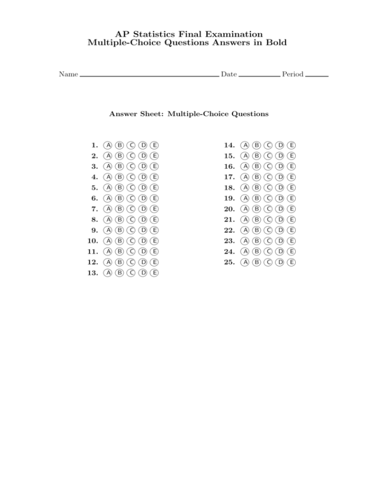
AP Statistics Final Examination
Multiple-Choice Questions Answers in Bold
Name
Date
Period
Answer Sheet: Multiple-Choice Questions
1.
l El
Al Bl Cl D
14.
l El
Al Bl Cl D
2.
l El
Al Bl Cl D
15.
l El
Al Bl Cl D
3.
l El
Al Bl Cl D
16.
l El
Al Bl Cl D
4.
l El
Al Bl Cl D
17.
l El
Al Bl Cl D
5.
l El
Al Bl Cl D
18.
l El
Al Bl Cl D
6.
l El
Al Bl Cl D
19.
l El
Al Bl Cl D
7.
l El
Al Bl Cl D
20.
l El
Al Bl Cl D
8.
l El
Al Bl Cl D
21.
l El
Al Bl Cl D
9.
l El
Al Bl Cl D
22.
l El
Al Bl Cl D
10.
l El
Al Bl Cl D
23.
l El
Al Bl Cl D
11.
l El
Al Bl Cl D
24.
l El
Al Bl Cl D
12.
l El
Al Bl Cl D
25.
l El
Al Bl Cl D
13.
l El
Al Bl Cl D
Formulas
I. Decriptive Statistics
P
xi
x =
rn
1 X
(x1 − x)2
sx =
n−1
s
(n1 − 1)s21 + (n2 − 1)s22
sp =
(n1 − 1) + (n2 − 1)
ŷ = b0 + b1 x
P
(x1 − x)(yi − y)
P
b1 =
(sx − x)2
b0 = y − b1 x
1 X x1 − x
yi − y
r =
n−1
sx
sy
sy
b1 = r
s
rxP
(yi − y)2
sb1 = pP n − 2
(xi − x)2
II. Probability
P (A ∩ B)
P (B)
P (A ∩ B)
P (A|B) =
P (B)
P
E(X) = µX = xi pi
P
Var(X) = σx2 = (xi − µX )2 pi
P (A ∪ B) =
If X has a binomial distribution with parameters n and p, then:
P (X = k) = nk pk (1 − p)n−k
µX = p
np
σX = np (1 − p)
µp̂ = p
r
p(1 − p)
σp̂ =
n
If x is the mean of a random sample of size n from an infinite population with
mean µ and standard deviation σ, the:
µx = µ
σ
σx = √
n
III. Inferential Statistics
Standardized test statistic:
statistic − parameter
standard deviation of statistic
Confidence interval:
statistic ± (critical value) · (standard deviation of statistic)
Single-Sample
Statistic
Standard Deviation
of Statistic
σ
√
n
r
p (1 − p)
n
Sample Mean
Sample Proportion
Two-Sample
Statistic
Standard Deviation
of Statistic
s
Difference of
sample means
σ12 σ22
+
n1 n2
Special case when σ1 = σ2
Difference of
sample proportions
r
1
1
σ
+
n1 n2
s
p1 (1 − p1 ) p2 (1 − p2 )
+
n1
n2
Special case when p1 = p2 = p
r
1
1
+
p (1 − p)
n1 n2
p
Chi − square test statistic =
X (observed = expected)2
expected
Appendix
580
Table entry
Table entry for z is the
area under the standard
normal curve left of z .
z
TABLE A Standard normal probabilities
z
.00
.01
.02
.03
.04
.05
.06
.07
.08
.09
23.4
23.3
23.2
23.1
23.0
22.9
22.8
22.7
22.6
22.5
22.4
22.3
22.2
22.1
22.0
21.9
21.8
21.7
21.6
21.5
21.4
21.3
21.2
21.1
21.0
20.9
20.8
20.7
20.6
20.5
20.4
20.3
20.2
20.1
20.0
.0003
.0005
.0007
.0010
.0013
.0019
.0026
.0035
.0047
.0062
.0082
.0107
.0139
.0179
.0228
.0287
.0359
.0446
.0548
.0668
.0808
.0968
.1151
.1357
.1587
.1841
.2119
.2420
.2743
.3085
.3446
.3821
.4207
.4602
.5000
.0003
.0005
.0007
.0009
.0013
.0018
.0025
.0034
.0045
.0060
.0080
.0104
.0136
.0174
.0222
.0281
.0351
.0436
.0537
.0655
.0793
.0951
.1131
.1335
.1562
.1814
.2090
.2389
.2709
.3050
.3409
.3783
.4168
.4562
.4960
.0003
.0005
.0006
.0009
.0013
.0018
.0024
.0033
.0044
.0059
.0078
.0102
.0132
.0170
.0217
.0274
.0344
.0427
.0526
.0643
.0778
.0934
.1112
.1314
.1539
.1788
.2061
.2358
.2676
.3015
.3372
.3745
.4129
.4522
.4920
.0003
.0004
.0006
.0009
.0012
.0017
.0023
.0032
.0043
.0057
.0075
.0099
.0129
.0166
.0212
.0268
.0336
.0418
.0516
.0630
.0764
.0918
.1093
.1292
.1515
.1762
.2033
.2327
.2643
.2981
.3336
.3707
.4090
.4483
.4880
.0003
.0004
.0006
.0008
.0012
.0016
.0023
.0031
.0041
.0055
.0073
.0096
.0125
.0162
.0207
.0262
.0329
.0409
.0505
.0618
.0749
.0901
.1075
.1271
.1492
.1736
.2005
.2296
.2611
.2946
.3300
.3669
.4052
.4443
.4840
.0003
.0004
.0006
.0008
.0011
.0016
.0022
.0030
.0040
.0054
.0071
.0094
.0122
.0158
.0202
.0256
.0322
.0401
.0495
.0606
.0735
.0885
.1056
.1251
.1469
.1711
.1977
.2266
.2578
.2912
.3264
.3632
.4013
.4404
.4801
.0003
.0004
.0006
.0008
.0011
.0015
.0021
.0029
.0039
.0052
.0069
.0091
.0119
.0154
.0197
.0250
.0314
.0392
.0485
.0594
.0721
.0869
.1038
.1230
.1446
.1685
.1949
.2236
.2546
.2877
.3228
.3594
.3974
.4364
.4761
.0003
.0004
.0005
.0008
.0011
.0015
.0021
.0028
.0038
.0051
.0068
.0089
.0116
.0150
.0192
.0244
.0307
.0384
.0475
.0582
.0708
.0853
.1020
.1210
.1423
.1660
.1922
.2206
.2514
.2843
.3192
.3557
.3936
.4325
.4721
.0003
.0004
.0005
.0007
.0010
.0014
.0020
.0027
.0037
.0049
.0066
.0087
.0113
.0146
.0188
.0239
.0301
.0375
.0465
.0571
.0694
.0838
.1003
.1190
.1401
.1635
.1894
.2177
.2483
.2810
.3156
.3520
.3897
.4286
.4681
.0002
.0003
.0005
.0007
.0010
.0014
.0019
.0026
.0036
.0048
.0064
.0084
.0110
.0143
.0183
.0233
.0294
.0367
.0455
.0559
.0681
.0823
.0985
.1170
.1379
.1611
.1867
.2148
.2451
.2776
.3121
.3483
.3859
.4247
.4641
Appendix
581
Table entry
!
"
#
$
%
%
&
'
(
)
*
+
(
,
-
'
.
%
5
"
(
&
%
"
+
+
/
(
1
*
&
"
0
$
%
2
(
/
'
(
.
3
%
-
%
'
'
+
"
'
&
.
0
%
"
$
(
0
%
*
'
z
4
5
TABLE A S t
z
c
.
Probability
p
Table entry for p and C is
the critical value t ⴱ with
probability p lying to its right
and probability C lying between
⫺t ⴱ and t ⴱ .
t*
TABLE C t distribution critical values
Upper tail probability p
df
.25
.20
.15
.10
.05
.025
.02
.01
.005
.0025
.001
.0005
1
2
3
4
5
6
7
8
9
10
11
12
13
14
15
16
17
18
19
20
21
22
23
24
25
26
27
28
29
30
40
50
60
80
100
1000
zⴱ
1.000
0.816
0.765
0.741
0.727
0.718
0.711
0.706
0.703
0.700
0.697
0.695
0.694
0.692
0.691
0.690
0.689
0.688
0.688
0.687
0.686
0.686
0.685
0.685
0.684
0.684
0.684
0.683
0.683
0.683
0.681
0.679
0.679
0.678
0.677
0.675
0.674
1.376
1.061
0.978
0.941
0.920
0.906
0.896
0.889
0.883
0.879
0.876
0.873
0.870
0.868
0.866
0.865
0.863
0.862
0.861
0.860
0.859
0.858
0.858
0.857
0.856
0.856
0.855
0.855
0.854
0.854
0.851
0.849
0.848
0.846
0.845
0.842
0.841
1.963
1.386
1.250
1.190
1.156
1.134
1.119
1.108
1.100
1.093
1.088
1.083
1.079
1.076
1.074
1.071
1.069
1.067
1.066
1.064
1.063
1.061
1.060
1.059
1.058
1.058
1.057
1.056
1.055
1.055
1.050
1.047
1.045
1.043
1.042
1.037
1.036
3.078
1.886
1.638
1.533
1.476
1.440
1.415
1.397
1.383
1.372
1.363
1.356
1.350
1.345
1.341
1.337
1.333
1.330
1.328
1.325
1.323
1.321
1.319
1.318
1.316
1.315
1.314
1.313
1.311
1.310
1.303
1.299
1.296
1.292
1.290
1.282
1.282
6.314
2.920
2.353
2.132
2.015
1.943
1.895
1.860
1.833
1.812
1.796
1.782
1.771
1.761
1.753
1.746
1.740
1.734
1.729
1.725
1.721
1.717
1.714
1.711
1.708
1.706
1.703
1.701
1.699
1.697
1.684
1.676
1.671
1.664
1.660
1.646
1.645
12.71
4.303
3.182
2.776
2.571
2.447
2.365
2.306
2.262
2.228
2.201
2.179
2.160
2.145
2.131
2.120
2.110
2.101
2.093
2.086
2.080
2.074
2.069
2.064
2.060
2.056
2.052
2.048
2.045
2.042
2.021
2.009
2.000
1.990
1.984
1.962
1.960
15.89
4.849
3.482
2.999
2.757
2.612
2.517
2.449
2.398
2.359
2.328
2.303
2.282
2.264
2.249
2.235
2.224
2.214
2.205
2.197
2.189
2.183
2.177
2.172
2.167
2.162
2.158
2.154
2.150
2.147
2.123
2.109
2.099
2.088
2.081
2.056
2.054
31.82
6.965
4.541
3.747
3.365
3.143
2.998
2.896
2.821
2.764
2.718
2.681
2.650
2.624
2.602
2.583
2.567
2.552
2.539
2.528
2.518
2.508
2.500
2.492
2.485
2.479
2.473
2.467
2.462
2.457
2.423
2.403
2.390
2.374
2.364
2.330
2.326
63.66
9.925
5.841
4.604
4.032
3.707
3.499
3.355
3.250
3.169
3.106
3.055
3.012
2.977
2.947
2.921
2.898
2.878
2.861
2.845
2.831
2.819
2.807
2.797
2.787
2.779
2.771
2.763
2.756
2.750
2.704
2.678
2.660
2.639
2.626
2.581
2.576
127.3
14.09
7.453
5.598
4.773
4.317
4.029
3.833
3.690
3.581
3.497
3.428
3.372
3.326
3.286
3.252
3.222
3.197
3.174
3.153
3.135
3.119
3.104
3.091
3.078
3.067
3.057
3.047
3.038
3.030
2.971
2.937
2.915
2.887
2.871
2.813
2.807
318.3
22.33
10.21
7.173
5.893
5.208
4.785
4.501
4.297
4.144
4.025
3.930
3.852
3.787
3.733
3.686
3.646
3.611
3.579
3.552
3.527
3.505
3.485
3.467
3.450
3.435
3.421
3.408
3.396
3.385
3.307
3.261
3.232
3.195
3.174
3.098
3.091
636.6
31.60
12.92
8.610
6.869
5.959
5.408
5.041
4.781
4.587
4.437
4.318
4.221
4.140
4.073
4.015
3.965
3.922
3.883
3.850
3.819
3.792
3.768
3.745
3.725
3.707
3.690
3.674
3.659
3.646
3.551
3.496
3.460
3.416
3.390
3.300
3.291
50%
60%
70%
80%
90%
95%
96%
98%
99%
99.5%
99.8%
99.9%
Confidence level C
583
588
Appendix
Probability p
Table entry for p is the
critical value x ⴱ with
probability p lying to its
right.
x*
TABLE E Chi-square distribution critical values
p
df
.25
.20
.15
.10
.05
.025
.02
.01
.005
.0025
.001
.0005
1
2
3
4
5
6
7
8
9
10
11
12
13
14
15
16
17
18
19
20
21
22
23
24
25
26
27
28
29
30
40
50
60
80
100
1.32
2.77
4.11
5.39
6.63
7.84
9.04
10.22
11.39
12.55
13.70
14.85
15.98
17.12
18.25
19.37
20.49
21.60
22.72
23.83
24.93
26.04
27.14
28.24
29.34
30.43
31.53
32.62
33.71
34.80
45.62
56.33
66.98
88.13
109.1
1.64
3.22
4.64
5.99
7.29
8.56
9.80
11.03
12.24
13.44
14.63
15.81
16.98
18.15
19.31
20.47
21.61
22.76
23.90
25.04
26.17
27.30
28.43
29.55
30.68
31.79
32.91
34.03
35.14
36.25
47.27
58.16
68.97
90.41
111.7
2.07
3.79
5.32
6.74
8.12
9.45
10.75
12.03
13.29
14.53
15.77
16.99
18.20
19.41
20.60
21.79
22.98
24.16
25.33
26.50
27.66
28.82
29.98
31.13
32.28
33.43
34.57
35.71
36.85
37.99
49.24
60.35
71.34
93.11
114.7
2.71
4.61
6.25
7.78
9.24
10.64
12.02
13.36
14.68
15.99
17.28
18.55
19.81
21.06
22.31
23.54
24.77
25.99
27.20
28.41
29.62
30.81
32.01
33.20
34.38
35.56
36.74
37.92
39.09
40.26
51.81
63.17
74.40
96.58
118.5
3.84
5.99
7.81
9.49
11.07
12.59
14.07
15.51
16.92
18.31
19.68
21.03
22.36
23.68
25.00
26.30
27.59
28.87
30.14
31.41
32.67
33.92
35.17
36.42
37.65
38.89
40.11
41.34
42.56
43.77
55.76
67.50
79.08
101.9
124.3
5.02
7.38
9.35
11.14
12.83
14.45
16.01
17.53
19.02
20.48
21.92
23.34
24.74
26.12
27.49
28.85
30.19
31.53
32.85
34.17
35.48
36.78
38.08
39.36
40.65
41.92
43.19
44.46
45.72
46.98
59.34
71.42
83.30
106.6
129.6
5.41
7.82
9.84
11.67
13.39
15.03
16.62
18.17
19.68
21.16
22.62
24.05
25.47
26.87
28.26
29.63
31.00
32.35
33.69
35.02
36.34
37.66
38.97
40.27
41.57
42.86
44.14
45.42
46.69
47.96
60.44
72.61
84.58
108.1
131.1
6.63
9.21
11.34
13.28
15.09
16.81
18.48
20.09
21.67
23.21
24.72
26.22
27.69
29.14
30.58
32.00
33.41
34.81
36.19
37.57
38.93
40.29
41.64
42.98
44.31
45.64
46.96
48.28
49.59
50.89
63.69
76.15
88.38
112.3
135.8
7.88
10.60
12.84
14.86
16.75
18.55
20.28
21.95
23.59
25.19
26.76
28.30
29.82
31.32
32.80
34.27
35.72
37.16
38.58
40.00
41.40
42.80
44.18
45.56
46.93
48.29
49.64
50.99
52.34
53.67
66.77
79.49
91.95
116.3
140.2
9.14
11.98
14.32
16.42
18.39
20.25
22.04
23.77
25.46
27.11
28.73
30.32
31.88
33.43
34.95
36.46
37.95
39.42
40.88
42.34
43.78
45.20
46.62
48.03
49.44
50.83
52.22
53.59
54.97
56.33
69.70
82.66
95.34
120.1
144.3
10.83
13.82
16.27
18.47
20.51
22.46
24.32
26.12
27.88
29.59
31.26
32.91
34.53
36.12
37.70
39.25
40.79
42.31
43.82
45.31
46.80
48.27
49.73
51.18
52.62
54.05
55.48
56.89
58.30
59.70
73.40
86.66
99.61
124.8
149.4
12.12
15.20
17.73
20.00
22.11
24.10
26.02
27.87
29.67
31.42
33.14
34.82
36.48
38.11
39.72
41.31
42.88
44.43
45.97
47.50
49.01
50.51
52.00
53.48
54.95
56.41
57.86
59.30
60.73
62.16
76.09
89.56
102.7
128.3
153.2
Section I
Questions 1–25
Directions: The questions or incomplete statements that follow are each followed by five
suggested answers or completions. Choose the response that best answers the question or
completes the statement.
1. Suppose there is a correlation of r = 0.9 between number of hours per day
students study and GPAs. Which of the following is a reasonable conclusion?
(A) 90% of students who study receive high grades.
(B) 90% of students who receive high grades study a lot.
(C) 90% of the variation in GPAs can be explained by variation in number of
study hours.
(D) 10% of the variation in GPAs cannot be explained by variation in number
of study hours per day.
(E) 81% of the variation in GPAs can be explained by variation in number of
study hours per day.
2. A pet food manufacturer runs an experiment to determine whether three brands
of dog food ae equally preferred by dogs. In the experiment, 150 dogs are individually presented with three dishes of food, each containing a different brand,
and their choices are noted. Tabulations show that 62 dogs go to brand A, 43 to
brand B, and 45 to brand C. Is there sufficient evidence to say that dogs have
preferences among the brands? Test at the 10% significance level.
(A) No, with χ2 = 2.09, there is not sufficient evidence even at the 25% significance level.
(B) No, with χ2 = 4.36, there is not sufficient evidence at the 10% level.
(C) No, with χ2 = 19.0, there is not sufficient evidence even at the 0.1% level.
(D) Yes, with χ2 = 4.36, there is sufficient evidence at the 10% level.
(E) Yes, with χ2 = 19.0, there is sufficient evidence even at the 0.1% level.
3. The American Medical Association (AMA) wishes to determine the percentage
of obstetricians who are considering leaving the profession because of the rapidly
increasing number of lawsuits against obstetricians. How large a sample should
be taken to find the answer to within ±3% at the 95% confidence level?
(A) 6
(B) 33
(C) 534
(D) 752
(E) 1068
4. Which of the following are true statements?
I. If there is sufficient evidence to reject a null hypothesis at the 10% level, then
there is sufficient evidence to reject it at the 5% level.
II. Whether to use a one- or two-sided test is typically decided after the data
are gathered.
III. If a hypothesis test is conducted at the 1% level, there is a 1% chance of
rejecting the null hypothesis.
(A) I only
(B) II only
(C) III only
(D) I, II, and III
(E) None are true.
5. A manufacturer claims that a particular automobile model will get 50 miles per
gallon on the highway. The researchers at a consumer-oriented magazine believe
that this claim is high and plan a test with a simple ramdom sample of 30 cars.
Assuming the standard deviation between individual cars is 2.3 miles per gallon,
what should the researchers conclude if the sample mean is 49 miles per gallon?
(A) There is not sufficient evidence to reject the manufacturer’s claim; 49 miles
per gallon is too close to the claimed 50 miles per gallon.
(B) The manufacturer’s claim should not be rejected because the P -value of
.0087 is too small.
(C) The manufacturer’s claim should be rejected because the sample mean is
less than the claimed mean.
(D) The P -value of .0087 is sufficient evidence to reject the manufacturer’s
claim.
(E) The P -value of .0087 is sufficient evidence to prove that the manufacturer’s
claim is false.
6. A historian believes that the average height of soldiers in World War II was
greater than that of soldiers in World War I. She examines a random sample
of records of 100 men in each war and notes standard deviations of 2.5 and 2.3
inches in World War I and World War II, respectively. If the average height from
the sample of World War II soldiers is 1 inch greater than from the sample of
World War I soldiers, what conclusion is justified from a two-sample hypothesis
test where
H0 : µ1 − µ2 = 0 and Ha : µ1 − µ2 < 0?
(A) The observed difference in average height is significant.
(B) The observed difference in average height is not significant.
(C) A conclusion is not possible without knowing the mean height in each
sample.
(D) A conclusion is not possible without knowing both the sample means and
the two original population sizes.
(E) A two-sample hypothesis test should not be used in this example.
7. Which of the following statements about the correlation coefficient are true?
I. The correlation coefficient and the slope of the regression line may have
opposite signs.
II. A correlation of 1 indicates a perfect cause-and-effect relationship between
the variables.
III. Correlations of +.87 and −.87 indicate the same degree of clustering around
the regression line.
(A) I only
(B) II only
(C) III only
(D) I and II
(E) I, II, and III
8. A soft drink dispenser can be adjusted to deliver any fixed number of ounces
of soft drink. If the machine is operating with a standard deviation in delivery
equal to 0.3 ounces, what should be the mean setting so that a 12-ounce cup
will overflow less then 1% of the time? Assume a normal distribution for ounces
delivered.
(A) 11.23 ounces
(B) 11.30 ounces
(C) 11.70 ounces
(D) 12.70 ounces
(E) 12.77 ounces
9. The death rate from a particular form of cancer is 23% during the first year.
When treated with an experimental drug, only 15 out of 84 patients die during
the initial year. Is this strong evidence to claim that the new medication reduces
the mortality rate?
(A) Yes, because the P -value is .0459.
(B) Yes, because the P -value is .1314.
(C) No, because the P -value is only .0459.
(D) No, because the P -value is above .10.
(E) An answer cannot be given without first knowing if a placebo was also used
and what the results were.
10. Consider the following back-to-back stemplot:
843
65210
92
7552
6
8541
90
0
1
2
3
4
5
6
7
8
9
348
01256
29
2557
6
1458
09
Which of the following are true statements?
I. The distributions have the same mean.
II. The distributions have the same range.
III. The distributions have the same standard deviation.
(A) II only
(B) I and II
(C) I and III
(D) II and III
(E) I, II, and III
11. A plumbing contractor obtains 60% of her boiler circulators from a company
whose defect rate is 0.005, and the rest from a company whose defect rate is
0.010. What proportion of the circulators can be expected to be defective?
If a circulator is defective, what is the probability that it came from the first
company?
(A) .0070, .429
(B) .0070, .600
(C) .0075, .500
(D) .0075, .600
(E) .0150, .571
12. The graph below shows cumulative proportions plotted against land values (in
dollars per acre) for farms on sale in a rural community.
1.0
Cumulative 0.8
production 0.6
0.4
0.2
1000
2000
3000
Dollars per acre
4000
What is the median land value?
(A) $2000
(B) $2250
(C) $2500
(D) $2750
(E) $3000
13. A teacher believes that giving her students a practice quiz every week will motivate them to study harder, leading to a greater overall understanding of the
course material. She tries this technique for a year, and everyone in the class
achieved a grade of a least C. Is this an experiment or an observational study?
(A) An experiment, but with no reasonable conclusion possible about cause
and effect
(B) An experiment, thus making cause and effect a reasonable conclusion
(C) An observational study, because there was no use of a control group
(D) An observational study, but a poorly designed one because randomization
was not used
(E) An observational study, and thus a reasonable conclusion of association but
not of cause and effect
14. In a simple random survey of 89 teachers of high school AP Statistics, 73 said
that it was the most satisfying, most enjoyable course they had ever taught.
Establish a 98% confidence interval estimate of the proportion of all high school
AP Statistics teachers who feel this way.
(A) .820 ± .004
(B) .820 ± .041
(C) .820 ± .084
(D) .820 ± .095
(E) .820 ± .223
15. To survey the opinions of the students at your high school, a researcher plans to
select every twenty-fifth student entering the school in the morning. Assuming
there are no absences, will this result in a simple random sample of students
attending your school?
(A) Yes, because every students has the same chance of being selected.
(B) Yes, but only if there is a single entrance to the school.
(C) Yes, because the 24 out of every 25 students who are not selected will form
a control group.
(D) Yes, because this is an example of systematic sampling, which is a special
case of simple random sampling.
(E) No, because not every sample of the intended size has an equal chance of
being selected.
16. Following is a histogram of ages of people applying for a particular high-school
teaching position.
21
22
23
24
25
26
27
28
Which of the following statements are true?
I. The median age is between 24 and 25.
II. The mean age is between 22 and 23.
III. The mean age is greater than the median age.
(A) I only
(B) II only
(C) III only
(D) All are true
(E) None is true
17. Suppose 4% of the population have a certain disease. A laboratory blood test
gives a positive reading for 95% of people who have the disease and for 5% of
people who do not have the disease. What is the probability of testing positive?
If a person tests positive, what is the probability the person has the disease?
(A) .086, .442
(B) .086, .500
(C) .086, .914
(D) .500, .950
(E) .914, .950
18. A reading specialist in a large public school system believes that the more time
students spend reading, the better they will do in school. She plans a middle
school experiment in which an SRS of 30 eighth graders will be assigned four
extra hours of reading per week, and SRS of 30 seventh graders will be assigned
two extra hours or reading per week, and an SRS of 30 sixth graders with no
extra assigned reading will be a control group. After one school year, the mean
GPAs from each group will be compared. Is this a good experimental design?
(A) Yes
(B) No, because while this design may point out an association between reading
and GPA, it cannot establish a cause-and-effect relationship.
(C) No, because without blinding, there is a strong chance of a placebo effect.
(D) No, because any conclusion would be flawed because of blocking bias.
(E) No, because grade level is a lurking variable which may well be confounded
with the variables under consideration.
19. To determine the mean cost of groceries in a certain city, an identical grocery
basket of food is purchased at each store in a random sample of ten stores. If the
average cost is $47.52 with a standard deviation of $1.59, find a 98% confidence
interval estimate for the cost of these groceries in the city.
(A) $47.52 ± $0.45
(B) $47.52 ± $1.17
(C) $47.52 ± $1.39
(D) $47.52 ± $1.42
(E) $47.52 ± $4.49
15
20. Suppose we have a random variable X where P (X = k) =
(.29)k (.71)15−k
k
for k = 0, 1, . . . , 15. What is the mean of X?
(A) 0.29
(B) 0.71
(C) 4.35
(D) 10.65
(E) None of the above
21. A study was conducted to determine the effectiveness of varying amounts of
vitamin C in reducing the number of common colds. A survey of 450 people
provided the following information:
Daily amount of vitamin C taken
None
500 mg
1000 mg
No colds
57
26
17
At least
one cold
223
84
43
Is there evidence of a relationship between catching a cold and taking vitamin
C?
(A) The data prove that vitamin C reduces the number of common colds.
(B) The data prove that vitamin C has no effect on the number of common
colds.
(C) There is sufficient evidence at the 1% significance level of a relationship
between taking vitamin C and catching fewer colds.
(D) There is sufficent evidence at the 10% significance level, but not at the 1%
significance level, of a relationship between taking vitamin C and catching
fewer colds.
(E) There is not sufficient evidence at the 10% level of a relationship between
takng vitamin C and catching fewer colds.
22. Both over-the-counter niacin and the prescription drug Lipitor are known to
lower blood cholesterol levels. In one double-blind study Lipitor outperformed
niacin. The 95% confidence interval estimate of the difference in mean cholesterol
level lowering was (18, 41). Which of the following is a reasonable conclusion?
(A) Niacin lowers cholesterol an average of 18 points, while Lipitor lowers cholesterol an average of 41 points.
(B) There is a .95 probability that Lipitor will outperform niacin in lowering
the cholesterol level of any given individual.
(C) There is a .95 probability that Lipitor will outperform niacin by at least 23
points in lowering the cholesterol level of any given individual.
(D) We should be 95% confident that Lipitor will outperform niacin as a
cholesterol-lowering drug.
(E) None of the above.
23. The boxpolts below summarize the distribution of SAT verbal and math scores
among students at an upstate New York high school.
Math:
Verbal:
300
400
500
600
700
Which of the following statements are true?
I. The range of the math scores equals the range of the verbal scores.
II. The highest math score equals the median verbal score.
III. The verbal scores appear to be roughly symmetric, while the math scores
appear to be skewed to the right.
(A) I only
(B) III only
(C) I and II
(D) II and III
(E) I, II, and III
24. A survey is conducted to determine the percentage of students at state universities who change their major at least once. In ans SRS of 100 students 78%
indicated that they graduated with a major different from the one with which
they entered college. Determine a 95% confidence interval for the percentage of
students who change their major.
(A) 68.2% to 87.8%
(B) 68.5% to 87.5%
(C) 69.9% to 86.1%
(D) 71.2% to 84.8%
(E) 73.9% to 82.1%
25. An Archaeopteryx is an extinct animal having feathers like a bird but also having
very prominent teeth. Five fossilized speciment of this creature have been found
with the lengths of the femur (a leg bone) plotted against the lengths of the
humerus (a bone in the upper arm):
Femur
38 56 59
64
74
Humerus
41 63 70
71
76
Archeologists have long felt that there should be a positive linear correlation
between the lengths of the femur and the lengths of the humerus in these extinct
creatures. What do the above data suggest?
(A) A positive correlation is likely because lengths of bones in any animal are
always positively correlated.
(B) A positive correlation is likely because the above test yields a P -value of
.0039.
(C) A positive correlation is likely because the above test yields a P -value of
.0078.
(D) There is no significant positive correlation at the 1% level of significance as
the P -value is .039.
(E) There is no significant positive correlation at the 5% level of significance as
the P -value is .078.
End of Multiple-Choice Questions