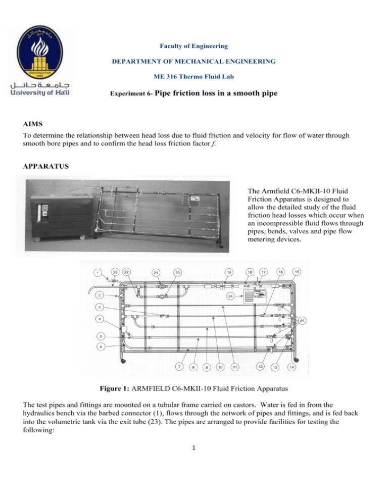
Faculty of Engineering
DEPARTMENT OF MECHANICAL ENGINEERING
ME 316 Thermo Fluid Lab
Experiment 6- Pipe
friction loss in a smooth pipe
AIMS
To determine the relationship between head loss due to fluid friction and velocity for flow of water through
smooth bore pipes and to confirm the head loss friction factor f.
APPARATUS
The Armfield C6-MKII-10 Fluid
Friction Apparatus is designed to
allow the detailed study of the fluid
friction head losses which occur when
an incompressible fluid flows through
pipes, bends, valves and pipe flow
metering devices.
Figure 1: ARMFIELD C6-MKII-10 Fluid Friction Apparatus
The test pipes and fittings are mounted on a tubular frame carried on castors. Water is fed in from the
hydraulics bench via the barbed connector (1), flows through the network of pipes and fittings, and is fed back
into the volumetric tank via the exit tube (23). The pipes are arranged to provide facilities for testing the
following:
1 • An in-line strainer (2)
• An artificially roughened pipe (7)
• Smooth bore pipes of 4 different diameters (8), (9),
(10) and (11)
• A long radius 90° bend (6)
• A short radius 90° bend (15)
• A 45° "Y" (4)
• A 45° elbow (5)
• A 90° "T" (13)
• A 90° mitre (14)
•
•
•
•
A 90° elbow (22)
A sudden contraction (3)
A sudden enlargement (16)
A pipe section made of clear acrylic with a Pitot static
tube (17)
A Venturi meter made of clear acrylic (18)
An orifice meter made of clear acrylic (19)
A ball valve (12)
A globe valve (20)
A gate valve (21)
•
•
•
•
•
SPECIFICATIONS
Test Pipe Diameters:
1.
19.1mm x 17.2mm
2.
12.7mm x 10.9mm
3.
9.5mm x 7.7mm
4.
6.4mm x 4.5mm
5.
19.1mmx 15.2mm (artificially roughened)
Distance between tapings: 1.00 m
BASIC THEORETICAL BACKGROUND
Two types of flow may exist in a pipe.
1)
Laminar flow at low velocities where h ∝ u
2)
Turbulent flow at higher velocities where h ∝ u n
Where h is the head loss due to friction and u is the fluid velocity:
For a circular pipe flowing full, the head loss due to friction may be calculated from the formula:
h=
2 fLu 2
(1)
gd
where: L is the length of the pipe between tapings, d is the internal diameter of the pipe,
u is the mean velocity of water through the pipe in m/s, g is the acceleration due to gravity
in m/s2 and f is the pipe friction coefficient.
The mean velocity is obtained from
u=
Reynolds' number, Re, is defined as: Re =
4Q
(2)
πd 2
ρud
μ
here Q is the volumetric flowrate in m3/s
(3)
where μ is the dynamic viscosity (1.15 x 10-3 Ns/m2 at 15°C) and ρ is the density (999 kg/m3 at 15°C).
2 The value of f may be determined as a function of Re and the relative roughness ε=e/d using a Moody diagram
(provided at the end of the handout).
Equation (1) can be used to determine the theoretical head loss by reading the value of f for the pipe in the
Moody diagram if you know Re and ε.
When h is measured experimentally, Eq. (1) can be rearranged to compute an experimental value for f.
f =
hgd
2Lu 2
(4)
PROCEDURE
1. Prime the pipe network with water. Open and close the appropriate valves to obtain flow of water through
the required test pipe.
2. Take readings at a number of different flow rates, altering the flow using the control valve on the apparatus,
(ten readings is sufficient to produce a good head-flow curve).
3. Measure flow rates using the volumetric tank. For small flow rates use the measuring cylinder. Measure
head loss between the tapings using the portable pressure meter or pressurized water manometer as
appropriate.
4. Obtain readings on all four smooth test pipes if you have the time.
REPORT
1. All readings should be tabulated in the table provided at the end of the handout:
2. Plot a graph of h (experimental) versus u for each size of pipe. Identify the laminar, transition and
turbulent zones on the graphs.
3. Confirm that the graph is a straight line for the zone of laminar flow h α u. Use the graph to determine
the critical Reynolds’ number for transition from laminar to turbulent flow.
4. Plot a graph of the experimental (direct reading) and calculated values of h (using Eq. 1 and the readings
of f from the Moody diagram) versus Re for all pipe diameters in the same graph and make a comparison
between the experimental and theoretical curves.
Note: be careful about the units so that you obtain h in m H2O
3 Table of readings and results
Volume
V
[litres]
Time
T
[Secs]
Flow
rate
Q
[m3/s]
Vx10-3
T
Pipe
Diam.
d
[m]
Velocity Reynolds
u
Number
[m/s]
Re
Eq.(2)
4 Eq.(3)
Measured
Head Loss
h
[m H2O]
(hC-hD)
Friction
factor
f
Moody
Diagram
Calculated
Head Loss
h
[m H2O]
Eq.(1)
Table of readings and results
Volume
V
[litres]
Time
T
[Secs]
Flow
rate
Q
[m3/s]
Vx10-3
T
Pipe
Diam.
d
[m]
Velocity Reynolds
u
Number
[m/s]
Re
Eq.(2)
5 Eq.(3)
Measured
Head Loss
h
[m H2O]
(hC-hD)
Friction
factor
f
Moody
Diagram
Calculated
Head Loss
h
[m H2O]
Eq.(1)
6