Worked examples — Multiple Random Variables
Example 1
Let X and Y be random variables that take on values from the set {−1, 0, 1}.
(a) Find a joint probability mass assignment for which X and Y are independent, and
confirm that X 2 and Y 2 are then also independent.
(b) Find a joint pmf assignment for which X and Y are not independent, but for which
X 2 and Y 2 are independent.
Solution
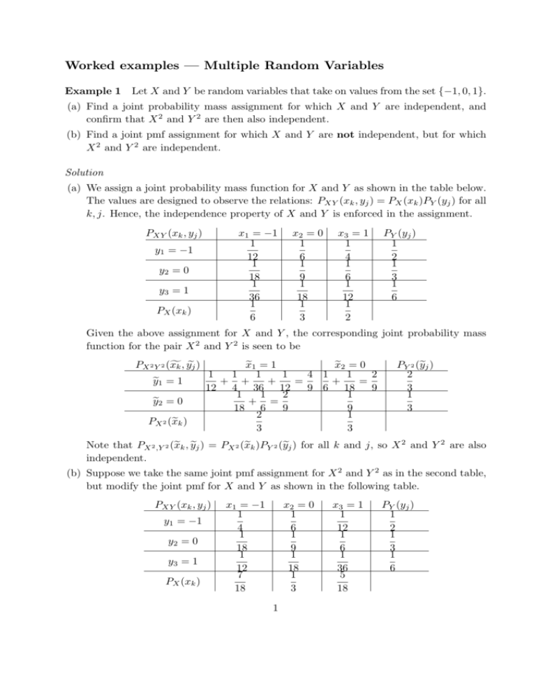
(a) We assign a joint probability mass function for X and Y as shown in the table below.
The values are designed to observe the relations: PXY (xk , yj ) = PX (xk )PY (yj ) for all
k, j. Hence, the independence property of X and Y is enforced in the assignment.
PXY (xk , yj )
x1 = −1
1
12
1
18
1
36
1
6
y1 = −1
y2 = 0
y3 = 1
PX (xk )
x2 = 0
1
6
1
9
1
18
1
3
x3 = 1
1
4
1
6
1
12
1
2
PY (yj )
1
2
1
3
1
6
Given the above assignment for X and Y , the corresponding joint probability mass
function for the pair X 2 and Y 2 is seen to be
PX 2 Y 2 (f
xk , yej )
ye1 = 1
ye2 = 0
PX 2 (e
xk )
x
e1 = 1
x
e2 = 0
1
1
1
1
4 1
1
2
+ +
+
=
+
=
12 4 36 12
9 6 18
9
1
1
2
1
+ =
18 6
9
9
2
1
3
3
PY 2 (e
yj )
2
3
1
3
Note that PX 2 ,Y 2 (e
xk , yej ) = PX 2 (e
xk )PY 2 (e
yj ) for all k and j, so X 2 and Y 2 are also
independent.
(b) Suppose we take the same joint pmf assignment for X 2 and Y 2 as in the second table,
but modify the joint pmf for X and Y as shown in the following table.
PXY (xk , yj )
y1 = −1
y2 = 0
y3 = 1
PX (xk )
x1 = −1
1
4
1
18
1
12
7
18
x2 = 0
1
6
1
9
1
18
1
3
1
x3 = 1
1
12
1
6
1
36
5
18
PY (yj )
1
2
1
3
1
6
This new joint pmf assignment for X and Y can be seen to give rise to the same joint
pmf assignment for X 2 and Y 2 in the second table. However, in this new assignment,
we observe that
1
7 1
7
= PXY (x1 , y1 ) 6= PX (x1 )PY (y1 ) =
· =
,
4
18 2
36
and the inequality of values can be observed also for PXY (x1 , y3 ), PXY (x3 , y1 ) and
PXY (x3 , y3 ), etc. Hence, X and Y are not independent.
Remark
1. Since −1 and 1 are the two positive square roots of 1, we have
PX (1) + PX (−1) = PX 2 (1) and
PY (1) + PY (−1) = PY 2 (1),
therefore
PX 2 (1)PY 2 (1) = [PX (1) + PX (−1)][PY (1) + PY (−1)]
= PX (1)PY (1) + PX (−1)PY (1) + PX (1)PY (−1) + PX (−1)PY (−1).
On the other hand, PX 2 Y 2 (1, 1) = PXY (1, 1) + PXY (−1, 1) + PXY (1, −1) + PXY
(−1, −1). Given that X 2 and Y 2 are independent, we have PX 2 Y 2 (1, 1) = PX 2 (1)
PY 2 (1), that is,
PXY (1, 1) + PXY (−1, 1) + PXY (1, −1) + PXY (−1, −1)
= PX (1)PY (1) + PX (−1)PY (1) + PX (1)PY (−1) + PX (−1)PY (−1).
However, there is no guarantee that PXY (1, 1) = PX (1)PY (1), PXY (1, −1) = PX (1)
PY (−1), etc., though their sums are equal.
2. Suppose X 3 and Y 3 are considered instead of X 2 and Y 2 . Can we construct a pmf
assignment where X 3 and Y 3 are independent but X and Y are not?
3. If the set of values assumed by X and Y is {0, 1, 2} instead of {−1, 0, 1}, can we
construct a pmf assignment for which X 2 and Y 2 are independent but X and Y are
not?
Example 2 Suppose the random variables X and Y have the joint density function
defined by
n
2 < x < 6, 0 < y < 5 .
f (x, y) = c(2x + y)
0
otherwise
(a) To find the constant c, we use
Z
6
Z
Z
5
1 = total probability =
5
c(2x + y) dydx =
Z
2
0
6
=
2
2
µ
¶ ¯5
y 2 ¯¯
c 2xy +
dx
2 ¯0
¶
µ
25
dx = 210c,
c 10x +
2
2
so c =
1
.
210
(b) The marginal cdf for X and Y are given by
Z
x
Z
∞
FX (x) = P (X ≤ x) =
f (x, y) dydx
−∞
0
Z




−∞
x
Z
5
2x + y
= Z2 Z 0 210
6
5


2x + y


210
2
0
Z ∞Z y
2x + y
FY (y) = P (Y ≤ y) =
−∞ −∞ 210

0 Z

Z

6
y


2x + y

= Z2 Z0 210

6
5

2x + y



210
2
0
2≤x<6
dydx = 1
x≥6
dydx
y<0
y 2 + 16y
dydx =
105
0≤y<5
dydx = 1
y≥5
½
4x+5
d
2 < x < 6.
84
(c) Marginal cdf for X: fX (x) =
FX (x) =
dx
0
otherwise
½
2y+16
d
0 < y < 5.
105
Marginal cdf for Y : fY (y) =
FY (y) =
dy
0
otherwise
Z 6Z 5
1
3
P (X > 3, Y > 2) =
(2x + y) dydx =
(d)
210 3 2
20
Z 6Z 5
1
23
P (X > 3) =
(2x + y) dydx =
210 3 0
28
Z 4 Z 4−x
1
2
P (X + Y < 4) =
(2x + y) dxdy =
210 2 0
35
3
x<2
2x2 + 5x − 18
dydx =
84
.
;
(e) Joint distribution function
y
F ( x, y )
5
=
F ( x, y ) = 0
F ( x, y ) = 0
2 x 2 + 5 x − 18
84
F ( x, y ) = 1
F ( x, y )
F ( x, y )
y 2 + 16 y
=
105
2 x 2 y + xy 2 − 8 y − 2 y 2
=
420
0
2
F ( x, y ) = 0
x
6
F ( x, y ) = 0
F ( x, y ) = 0
Suppose (x, y) is located in {(x, y) : x > 6, 0 < y < 5}, then
Z 6Z y
2x + y
y 2 + 16y
F (x, y) =
dydx =
,
210
105
2
0
2y + 16
.
105
Note that for this density f (x, y), we have
and f (x, y) =
f (x, y) 6= fX (x)fY (y),
so x and Y are not independent.
Example 3
The joint density of X and Y is given by
(
15
x(2 − x − y)
0 < x < 1, 0 < y < 1 .
f (x, y) =
2
0
otherwise
Compute the condition density of X, given that Y = y, where 0 < y < 1.
Solution
For 0 < x < 1, 0 < y < 1, we have
fX (x|y) =
f (x, y)
f (x, y)
= R∞
fY (y)
f (x, y) dx
−∞
= R1
0
Example 4
x(2 − x − y)
x(2 − x − y) dx
=
x(2 − x − y)
6x(2 − x − y)
=
.
y
2
4 − 3y
3 − 2
If X and Y have the joint density function
(
3
0 < x < 1, 0 < y < 1
fXY (x, y) = 4 + xy
0
otherwise
4
find (a) fY (y|x),
µ
¶
1 1
1
(b) P Y > | < X < + dx .
2 2
2
Solution
(a) For 0 < x < 1,
Z
1
fX (x) =
0
and
µ
3
+ xy
4
fXY (x, y)
fY (y|x) =
=
fX (x)
½
¶
dy =
3+4xy
3+2x
0
3 x
+
4 2
0<y<1.
otherwise
For other values of x, f (y|x) is not defined.
¯
¶ Z ∞
µ
µ
¶
Z 1
1
9
1 ¯¯ 1
1
3 + 2y
(b) P Y > ¯ < X < + dx =
fY y|
dy =
dy =
.
2 2
2
2
4
16
1/2
1/2
Example 5 Let X and Y be independent exponential random variables with parameter
α and β, respectively. Consider the square with corners (0, 0), (0, a), (a, a) and (a, 0), that
is, the length of each side is a.
y
(0, a)
(a, a)
(0, 0)
(a, 0)
x
(a) Find the value of a for which the probability that (X, Y ) falls inside a square of side
a is 1/2.
(b) Find the conditional pdf of (X, Y ) given that X ≥ a and Y ≥ a.
Solution
(a) The density function of X and Y are given by
½
½
−αx
βe−βy ,
y≥0
αe
,
x
≥
0
.
fX (x) =
, fY (y) =
0
y<0
0
x<0
Since X and Y are independent, so fXY (x, y) = fX (x)fY (y). Next, we compute
Z
a
Z
P [0 ≤ X ≤ a, 0 ≤ Y ≤ a] =
0
a
αβe−αx e−βy dxdy = (1 − e−aα )(1 − e−aβ ),
0
5
and solve for a such that (1 − e−aα )(1 − e−aβ ) = 1/2.
(b) Consider the following conditional pdf of (X, Y )
FXY (x, y|X ≥ a, Y ≥ a)
= P [X ≤ x, Y ≤ y|X ≥ a, Y ≥ a]
=
P [a ≤ X ≤ x, a ≤ Y ≤ y]
P [X ≥ a, Y ≥ a]
P [a ≤ X ≤ x]P [a ≤ Y ≤ y]
since X and Y are independent
P [X ≥ a]P [Y ≥ a]
 RyRx
 a a αβe−αx e−βy dxdy
(e−aα − e−αx )(e−aβ − e−βy )
R
R
=
,
∞ ∞
=
−αx e−βy dxdy
e−aα e−aβ
 a a αβe
0
=
x > a, y > a .
otherwise
∂2
FXY (x, y|X ≥ a, Y ≥ a)
∂x∂y
½
−αx −βy −αa −βa
e
/e
e
for x > a, y > a .
= αβe
0
otherwise
fXY (x, y|X ≥ a, Y ≥ a) =
Example 6 A point is chosen uniformly at random from the triangle that is formed by
joining the three points (0, 0), (0, 1) and (1, 0) (units measured in centimetre). Let X and
Y be the co-ordinates of a randomly chosen point.
(i) What is the joint density of X and Y ?
(ii) Calculate the expected value of X and Y , i.e., expected co-ordinates of a randomly
chosen point.
(iii) Find the correlation between X and Y . Would the correlation change if the units are
measured in inches?
Solution
(i) fX,Y (x, y) =
Z
1
= 2,
Area 4
∞
(ii) fX (x) =
0
(x, y) lies in the triangle.
Z
0
1−x
fX,Y (x, y ) dy =
−∞
Z ∞
fY (y) =
fX,Y (x0 , y) dx0 =
−∞
2 dy = 2(1 − x).
0
Z 1−y
2 dx = 2(1 − y).
0
Z
1
Hence, E[X] = 2
0
·
x2
x3
x(1 − x) dx = 2
−
2
3
6
¸1
=
0
1
3
Z
and E[Y ] = 2
1
1
.
3
y(1 − y) dy =
0
(iii) To find the correlation between X and Y , we consider
Z
1
Z
Z
1−y
E[XY ] = 2
xy dxdy = 2
0
1
Z
0
0
1
·
x2
y
2
¸1−y
dy
0
y(1 − 2y + y 2 ) dy
=
·
0
¸1
y2
2
y4
=
− y3 +
2
3
4
=
0
1
.
12
COV(X, Y ) = E[XY ] − E[X]E[Y ]
µ ¶2
1
1
1
=
−
=− .
12
3
36
· 3
¸1
Z 1
x
x4
1
2
2
E[X ] = 2
x (1 − x) dx = 2
−
=
3
4 0
6
0
so
1
VAR(X) = E[X ] − [E[X]] = −
6
2
Similarly, we obtain VAR(Y ) =
2
µ ¶2
1
1
=
.
3
18
1
.
18
−1
COV(X, Y )
1
p
ρXY = p
= 136 = − .
2
VAR(X) VAR(Y )
18
COV(aX, bY )
abCOV(X, Y )
=
= ρ(X, Y ), for any scalar multiσ(aX)σ(bY )
aσ(X)bσ(Y )
ples a and b. Therefore, the correlation would not change if the units are measured in
inches.
Since ρ(aX, bY ) =
Example 7 Let X, Y, Z be independent and uniformly distributed over (0, 1). Compute
P {X ≥ Y Z}.
Solution
Since X, Y, Z are independent, we have
fX,Y,Z (x, y, z) = fX (x)fY (y)fZ (z) = 1,
7
0 ≤ x ≤ 1, 0 ≤ y ≤ 1, 0 ≤ z ≤ 1.
Therefore,
ZZZ
P [X ≥ Y Z] =
fX,Y,Z (x, y, z) dxdydz
x≥yz
Z
1
Z
1
Z
=
1
Z
1
dxdydz =
0
Z
0
1
yz
³
1−
=
0
Example 8
Z
1
(1 − yz) dydz
0
0
z´
3
dz = .
2
4
The joint density of X and Y is given by
½
f (x, y) =
e−(x+y)
0
0 < x < ∞, 0 < y < ∞ .
otherwise
Find the density function of the random variable X/Y .
Solution
We start by computing the distribution function of X/Y . For a > 0,
·
¸
X
FX/Y (a) = P
≤a
Y
Z Z
Z
−(x+y)
=
e
dxdy =
0
x/y≤a
Z
∞
=
(1 − e
−ay
)e
−y
0
=1−
∞
Z
ay
e−(x+y) dxdy
0
·
¸ ¯∞
e−(a+1)y ¯¯
−y
dy = −e +
¯
a+1
0
a
1
=
.
a+1
a+1
By differentiating FX/Y (a) with respect to a, the density function X/Y is given by
fX/Y (a) = 1/(a + 1)2 , 0 < a < ∞.
Example 9 Let X and Y be a pair of independent random variables, where X is uniformly distributed in the interval (−1, 1) and Y is uniformly distributed in the interval
(−4, −1). Find the pdf of Z = XY .
8
Solution
Assume Y µ= y, then
of X. Suppose U = αW + β,
¶ Z = XY is a scaled version
µ ¯ ¶
1
u−β
1
z ¯¯
then fU (u) =
fW
. Now, fZ (z|y) =
fX
y ; the pdf of z is given by
|α|
α
|y|
y¯
µ ¯ ¶
µ
¶
Z ∞
Z ∞
1
z ¯¯
1
z
fZ (z) =
fX
y fY (y) dy =
fXY
, y dy.
y¯
y
−∞ |y|
−∞ |y|
½
1
−1 < x < 1 . Similarly, Y
Since X is uniformly distributed over (−1, 1), fX (x) = 2
0
otherwise
½
1
−4 < y < −1 . As X and Y are
is uniformly distributed over (−4, −1), fY (y) = 3
0
otherwise
independent,
(
¶
µ
µ ¶
z
1
z
z
−1 < < 1 and −4 < y < −1
fXY
, y = fX
fY (y) = 6
.
y
y
y
0
otherwise
We need to observe −1 < z/y < 1, which is equivalent to |z| < |y|. Consider the following
cases:
¶
µ
z
, y = 0.
(i) |z| > 4; now −1 < z/y < 1 is never satisfied so that fXY
y
(ii) |z| < 1; in this case, −1 < z/y < 1 is automatically satisfied so that
Z
−1
fZ (z) =
−4
1 1
dy =
|y| 6
µ
(iii) 1 < |z| < 4; note that fXY
Z
z
,y
y
−|z|
fZ (z) =
−4
¶
=
Z
−4
1
1
−
dy = − ln |y|
6y
6
¸−1
=
−4
ln 4
.
6
1
only for −4 < y < −|z|, so that
6
#−|z|
1 1
1
1
dy = − ln |y|
= [ln 4 − ln |z|].
|y| 6
6
6
−4

ln 4


 6
In summary, fZ (z) = 1

[ln 4 − ln |z|]

6
0
Z ∞
Z −1
Remark Check that
fZ (z) dz =
−∞
−1
if |z| < 1
if 1 < |z| < 4
otherwise
.
1
[ln 4 − ln |z|] dz
−4 6
Z 1
Z 4
ln 4
1
+
dz +
[ln 4 − ln |z|] dz
−1 6
1 6
Z 4
Z 4
ln 4
ln |z|
=
dz − 2
dz
6
−4 6
1
9
=
8
1
ln 4 − [z ln z − z]41 = 1.
6
3
Example 10 Let X and Y be two independent Gaussian random variables with zero
mean and unit variance. Find the pdf of Z = |X − Y |.
Solution We try to find FZ (z) = P [Z ≤ z]. Note that z ≥ 0 since Z is a non-negative
random variable.
y
Z=Y−X
when y > x
Z=X−Y
when x > y
x
Consider the two separate cases: x > y and x < y. When X = Y , Z is identically zero.
(i) x > y, Z ≤ z ⇔ x − y ≤ z, z ≥ 0; that is, x − z ≤ y < x.
y
Z=Y−X
when y > x
Z=X−Y
when x > y
x
x
×
x
×
x−z
x−z≤y<x
Z
∞
Z
x
FZ (z) =
fXY (x, y) dydx
−∞
x−z
Z ∞
d
fZ (z) =
FZ (z) =
fXY (x, x − z) dx
dz
−∞
Z ∞
1 −[x2 +(x−z)2 ]/2
e
dx
=
−∞ 2π
Z
2
1 −z2 /4 ∞ 1 −(x− z2 )2
1
√ e
= √ e
dx = √ e−z /4 .
2 π
π
2 π
−∞
10
(ii) x < y, Z ≤ z ⇔ y − x ≤ z, z ≥ 0; that is x < y ≤ x + z.
Z ∞ Z x+z
FZ (z) =
fXY (x, y) dydx
−∞
∞
Z
x
2
1
fZ (z) =
fXY (x, x + z) dx = √ e−z /4
2 π
−∞
Z
∞
−∞
2
2
1
1
√ e−(x+z) dx = √ e−z /4 .
π
2 π
Example 11 Suppose two persons A and B come to two separate counters for service.
Let their service times be independent exponential random variables with parameters λA
and λB , respectively. Find the probability that B leaves before A?
Solution
Let TA and TB denote the continuous random service time of A and B, re1
spectively. Recall that the expected value of the service times are: E[TA ] =
and
λA
1
E[TB ] =
. That is, a higher value of λ implies a shorter average service time. One
λB
would expect
P [TA > TB ] : P [TB > TA ] =
1
1
:
;
λA λB
and together with P [TA > TB ] + P [TB > TA ] = 1, we obtain
P [TA > TB ] =
λB
λA + λB
and
P [TB > TA ] =
λA
.
λA + λB
Justification:- Since TA and TB are independent exponential random variables, their joint
density fTA ,TB (tA , tB ) is given by
fTA ,TB (tA , tB ) dtA dtB
= P [tA < TA < tA + dtA , tB < TB < tB + dtB ]
= P [tA < TA < tA + dtA ]P [tB < TB < tB + dtB ]
= (λA e−λA tA dtA )(λB e−λB tB dtB ).
Z
∞
Z
tA
P [TA > TB ] =
Z
0
λA λB e−λA tA e−λB tB dtB dtA
0
∞
λA e−λA tA (1 − e−λB tA ) dtA
0
Z ∞
Z ∞
−λA tA
=
λA e
dtA −
λA e−(λA +λB )tA dtA
=
0
0
λB
λA
=
.
=1−
λA + λB
λA + λB
11
12