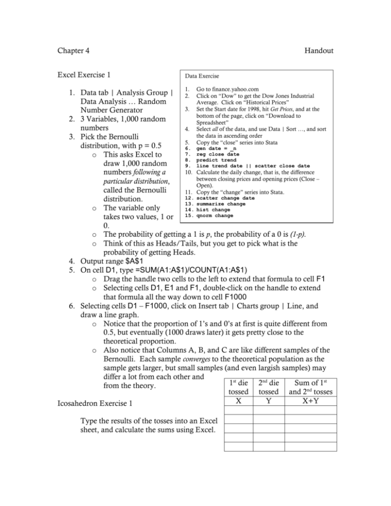
Chapter 4
Excel Exercise 1
Handout
Data Exercise
1.
Go to finance.yahoo.com
1. Data tab | Analysis Group | 2. Click on “Dow” to get the Dow Jones Industrial
Data Analysis … Random
Average. Click on “Historical Prices”
3.
Set the Start date for 1998, hit Get Prices, and at the
Number Generator
bottom of the page, click on “Download to
2. 3 Variables, 1,000 random
Spreadsheet”
numbers
4. Select all of the data, and use Data | Sort …, and sort
the data in ascending order
3. Pick the Bernoulli
5. Copy the “close” series into Stata
distribution, with p = 0.5
6. gen date = _n
7. reg close date
o This asks Excel to
8. predict trend
draw 1,000 random
9. line trend date || scatter close date
10. Calculate the daily change, that is, the difference
numbers following a
between closing prices and opening prices (Close –
particular distribution,
Open).
called the Bernoulli
11. Copy the “change” series into Stata.
12. scatter change date
distribution.
13. summarize change
o The variable only
14. hist change
15. qnorm change
takes two values, 1 or
0.
o The probability of getting a 1 is p, the probability of a 0 is (1-p).
o Think of this as Heads/Tails, but you get to pick what is the
probability of getting Heads.
4. Output range $A$1
5. On cell D1, type =SUM(A1:A$1)/COUNT(A1:A$1)
o Drag the handle two cells to the left to extend that formula to cell F1
o Selecting cells D1, E1 and F1, double-click on the handle to extend
that formula all the way down to cell F1000
6. Selecting cells D1 – F1000, click on Insert tab | Charts group | Line, and
draw a line graph.
o Notice that the proportion of 1’s and 0’s at first is quite different from
0.5, but eventually (1000 draws later) it gets pretty close to the
theoretical proportion.
o Also notice that Columns A, B, and C are like different samples of the
Bernoulli. Each sample converges to the theoretical population as the
sample gets larger, but small samples (and even largish samples) may
differ a lot from each other and
1st die 2nd die
Sum of 1st
from the theory.
tossed tossed and 2nd tosses
X
Y
X+Y
Icosahedron Exercise 1
Type the results of the tosses into an Excel
sheet, and calculate the sums using Excel.
A random American household will have X people living in it. If we ignore the
households were X > 7 (more that seven people live in that household), the
probability model for X is given by the following table
# of people in a household
X
1
2
3
4
5
6
7
P(X)
0.25
0.32
0.17
0.15
0.07
0.03
0.01
Given the information above, calculate the expected value, X = _______________.
Icosahedron Exercise 2
Calculate the theoretical expected value of the icosahedron
1. Make a column of 1, 2, 3, … 20
2. Make a column of the probability of each side of the icosahedron (1/20)
3. Multiply column 1 times column 2
4. Sum the third column
Icosahedron Exercise 3
Calculate empirical expected values of tosses of the icosahedron:
Use Excel for the calculations
Average of 1st toss
Average of 2nd toss
 X Y   X  Y
Average of 1 toss + Average of 2nd toss
Average of (1st + 2 toss)
st
1. Calculate  2Y 3  2Y  3 = ___________
Multiply each of the values of the 2nd toss times 2, then add 3 to each of the
results. Then take the average.
Or, multiply the average of the 2nd toss times 2. Add 3 to the result.
2.  X 2Y   X  2Y =_________
Multiply the values of the 2nd toss times 2, then add the value of the first toss
to each of the results, then take the average.
Multiply the average of the 2nd toss times 2. Add the average of the 1st toss to
the result.
Icosahedron Exercise 4
Calculate the theoretical standard deviation of
the icosahedron:
Compute the squared deviations,
multiply them times the probability, add
and then take the square root of the
result.
Icosahedron Exercise 5
Calculate empirical standard deviations of tosses of the icosahedron:
Variance of 1st toss
Standard deviation of 1st toss
Variance of 2nd toss
Standard deviation of 2nd toss
3.  2Y 3  2 Y
Multiply the 2nd toss-standard deviation times 2 = ______
Multiply the values of the 2nd toss times 2, then add 3 to each of the results. Then
calculate the standard deviation of the result = _____
4.  22Y 3  2 2  Y2
Multiply the 2nd toss-variance times (2)2 = ______
Multiply the values of the 2nd toss times 2, then add 3 to each of the results. The
variance of the result = _____
In Excel, calculate the correlation between the two tosses = _______.
5.  X2 Y   X2   Y2
Add the 1st toss variance to the 2nd toss variance = _______
Add the 1st toss values to the 2nd toss values. The variance of the result = _______
6.  X2  Y   X2   Y2
Add the 1st toss variance to the 2nd toss variance = _______
Subtract the values of the 1st toss from the values of the 2nd toss. The variance of the
result = _______
IF the two tosses were perfectly uncorrelated (correlation = 0), then the variance of
the sums should be exactly equal to the variance of the difference, and also equal to
the sum of the variances.
If the correlation is not 0, then
 X2 Y   X2   Y2  2  X  Y
 X2 Y   X2   Y2  2  X  Y
Icosahedron Exercise 6
7. If the correlation is not 0, you need to do something more. Using the
standard deviations you found above, multiply them, multiply the result times
the correlation, and multiply the total times 2.
2 X  Y = ______
 X2 Y
 X2   Y2  2  X  Y
 X2 Y
 X2   Y2  2 X  Y
Excel Exercise 2
1.
2.
3.
4.
5.
Tools | Data Analysis … | Random Number Generator
20 Variables, 1,000 random numbers
Pick the Normal distribution, with Mean = 0 and Standard Deviation = 1
Output range $D$9
Then do these calculations
Extended: Generate 200 Variables, 10,000 random numbers, with the
Bernoulli distribution, with p = 0.5
1.
2.
3.
From the above, copy the numbers of “avg1, “avg2”, etc.”
In a different sheet, open Edit | Paste Special … and select “Values” and “Transpose”
Label the columns
4.
copy everything and paste into STATA
5.
6.
7.
8.
9.
10.
11.
12.
13.
14.
hist five
hist twenty
hist onehundred
hist fivehundred
hist thousand
qnorm five
qnorm twenty
qnorm onehundred
qnorm fivehundred
qnorm thousand
five
twenty
fifty
hundred
fivehundred
thousand
Stata Exercise
1.
2.
set obs 250
gen x =
invnorm(uniform())
3. sum x in 1/60
4. sum x in 61/120
5. sum x in 121/180
6. sum x in 181/240
7. hist x in 1/60
8. hist x in 61/120
9. hist x in 121/180
10. hist x in 181/240