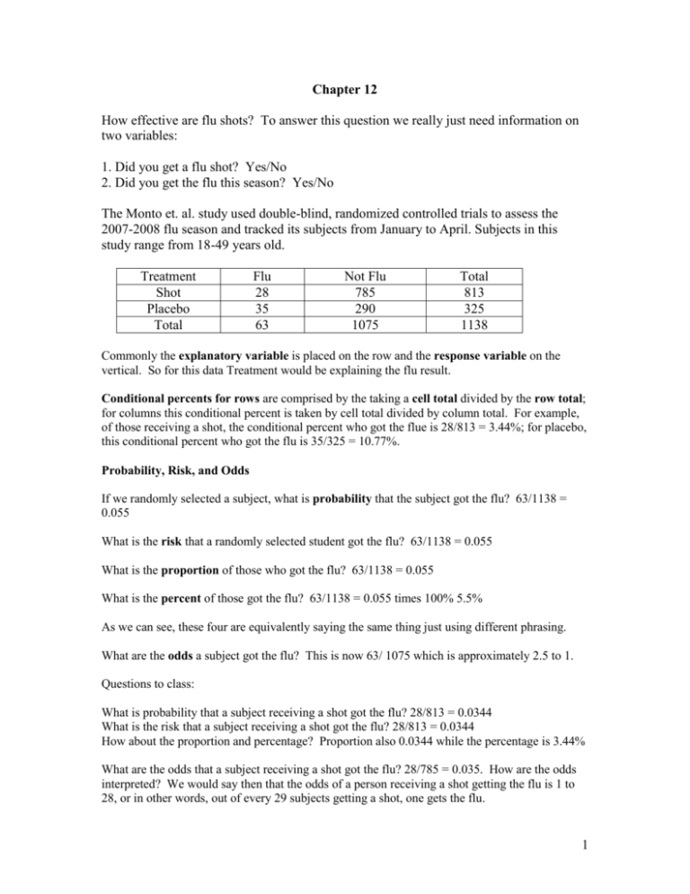
Chapter 12
How effective are flu shots? To answer this question we really just need information on
two variables:
1. Did you get a flu shot? Yes/No
2. Did you get the flu this season? Yes/No
The Monto et. al. study used double-blind, randomized controlled trials to assess the
2007-2008 flu season and tracked its subjects from January to April. Subjects in this
study range from 18-49 years old.
Treatment
Shot
Placebo
Total
Flu
28
35
63
Not Flu
785
290
1075
Total
813
325
1138
Commonly the explanatory variable is placed on the row and the response variable on the
vertical. So for this data Treatment would be explaining the flu result.
Conditional percents for rows are comprised by the taking a cell total divided by the row total;
for columns this conditional percent is taken by cell total divided by column total. For example,
of those receiving a shot, the conditional percent who got the flue is 28/813 = 3.44%; for placebo,
this conditional percent who got the flu is 35/325 = 10.77%.
Probability, Risk, and Odds
If we randomly selected a subject, what is probability that the subject got the flu? 63/1138 =
0.055
What is the risk that a randomly selected student got the flu? 63/1138 = 0.055
What is the proportion of those who got the flu? 63/1138 = 0.055
What is the percent of those got the flu? 63/1138 = 0.055 times 100% 5.5%
As we can see, these four are equivalently saying the same thing just using different phrasing.
What are the odds a subject got the flu? This is now 63/ 1075 which is approximately 2.5 to 1.
Questions to class:
What is probability that a subject receiving a shot got the flu? 28/813 = 0.0344
What is the risk that a subject receiving a shot got the flu? 28/813 = 0.0344
How about the proportion and percentage? Proportion also 0.0344 while the percentage is 3.44%
What are the odds that a subject receiving a shot got the flu? 28/785 = 0.035. How are the odds
interpreted? We would say then that the odds of a person receiving a shot getting the flu is 1 to
28, or in other words, out of every 29 subjects getting a shot, one gets the flu.
1
Relative Risk is when two risks are compared. For instance the relative risk that "those receiving
the shot get the flu" to "those receiving the placebo get the flu." The Shot-Flu risk is 28/813 and
the Placebo-Flu risk is 35/325. This would make the relative risk (28/813)/(35/325). This
computes to 0.0344/0.108 = 0.32 or about 1/3 The interpretation is that the risk of getting the
flu for those who took the shot is is about 1/3 less likely than for those getting the placebo.
Conversely, those receiving the placebo are at about three times greater risk (i.e 3 times more
likely) of getting the flu than those who received a shot.
Baseline risk is the risk to which another risk is compared to in a relative risk. That is it is the
risk in the denominator of the relative risk. In the previous example, "risk of those receiving the
shot getting the flu" was compared to the "risk of those receiving the placebo getting the flu"
making the placebo-flu risk the denominator. This makes the baseline risk the "risk of those
receiving the placebo getting the flu" or 0.108
Odds ratio is similar to relative risk except it is the ratio of two odds. The odds ratio that "those
receiving the shot get the flu" to "those receiving the placebo get the flu" is (28/785)/ (35/290) =
0.036/0.121 = 0.3 meaning for about every one person who receives placebo then gets the flu
about 0.3 people receiving the shot will get the flu.
Important To Interpret
When reading a report that provides a risk it is extremely important to know or be given the
baseline risk. For instance, say a study reported that women who binge drink are 3 times more
likely to develop liver disease than women who do not drink. This may alarm some females,
understandably. But what if the risk of getting liver disease for women who do not binge drink
(i.e. the baseline risk) was 0.001 or 1 out of a 1000 women who do not binge drink are likely to
develop liver disease. This would mean that risk of females who do binge drink developing liver
disease is 3/1000 or 0.003 Not that alarming!
Apply that to our flu discussion that has a Relative Risk of 0.32 or 1/3 meaning that those
receiving the shot are roughly 1/3 less likely to get the flu compared to those getting the placebo
(i.e. not the shot). However, the risk of getting the flu – i.e. the baseline risk – is 0.108.
Another way to look at this is that those not getting the shot have about a 10.8% chance of getting
the flu, while those receiving the shot have a 3.4% chance of getting the flu. Thus the flu shot
reduces the chance you get the flu by 7.4% This 7.4% percent reduction does not come across as
impressive as a 1/3 less chance. So what do you think: should you get the flu shot?
To calculate:
Odds are the (number of interest with trait)/(number of interest without trait)
Risk is the (number of interest with trait)/(over total number of interest)
2
Chapter 13
Ho: The two variables are not related in population (i.e. they are independent)
Ha: The two variables are related in the population (i.e. they are dependent)
Keeping with our flu discussion, this makes the hypotheses:
Ho: Receiving the flu shot and getting the flu are not related in the population
Ha: Receiving the flu shot and getting the flu are related in the population
What will indicate a relationship is a change in direction in the conditional percents from one
level of the explanatory to another level. But what determines HOW Different?
We apply what is called a Chi-square Test of Independence. This is done by first taking the
observed values to compute what you would expect to see if the two variables were independent.
This is done by creating expected counts in each cell of the table by using the row and column
tables compared to the overall total.
Finding Expected Table (i.e. based on the data collected, these are the counts we would
expect to find if the variables were independent – I'm just illustrating this, you won't be
responsible for actually doing these caclulations.)
Shot
Placebo
Total
Flu
(813x63)/1138
= 45
(325x63)/1138
= 18
63
No Flu
(813x1075)/1138
= 768
(325x1075)/1138
= 307
Total
813
1075
1138
325
This computes to, if independent, we would expect to see conditional percentages for Flu for of
5.5% (found by 45/813 and 18/325) and for No Flu of 94.5% (by 768/813 and 307/325)
The next step is to statistical compare what we would observed to what we expected. To do this
we calculate a chi-square test statistic and associated p-value (for this class the p-value will be
provided).
The general formula is: 
2
 (Observed  Expectect)

2
Expected
Applying that to this data:
C2 =
(28 - 45)2 (785- 768)2 (35-18)2 (290 - 307)2
=
=
=
=16
45
768
18
307
The p-value for this comes to approximately 0.000
Decision and conclusion: As with the test for a correlation the p-value is the probability the
sample data would produce a result given the null hypothesis is true. If the p-value is small then
this indicates that the variables are related. Again will use 0.05 as a level of significance to
compare with our p-value. Here the p-value of 0.000 is less than 0.05 so we reject the null
hypothesis and conclude that "flu shot and getting the flu" are related. Furthermore, we will
3
conclude that the chances or getting the flu are less likely for those who receive the shot than
those who do not.
NOTE: Keep in mind that the results can only be extended to sample group unless the data was
randomly selected and we cannot conclude a causal relationship unless random assignment was
involve. However, in this flu study with random assignment we can conclude cause although the
subjects were not sampled randomly.
Affect of Confounding Variables in Categorical Data Relationships
When a confounding variable is present (i.e. an explanatory variable that is related to another
explanatory variable plus the response variable) the statistical results may not reflect the true
relationship. This can lead to what is called Simpson’s Paradox
Simpson’s Paradox occurs when combined data leads to one result but when we separate the data
by another lurking variable we get opposite results.
Example: Following a 1972 Supreme Court ruling to eliminate racial disparities in capital cases,
several studies were conducted to follow-up on sentences of those found guilty of capital
offenses. One such study considered homicides in Florida between 1976 and 1977 to examine if
a relationship existed between race and assignment of the death penalty (see Michael Ravelet,
American Sociological Review, 1981 vol. 46).
Overall table:
Defendant/Death Penalty
White
Black
Total
NO
141
149
290
Yes
19
17
36
Total
160
166
326
% Yes
11.9%
10.2%
From this table it shows that White defendants that were guilty were slightly more likely to get
the death penalty than Black guilty defendants.
However, a lurking variable victim’s race provides a different look:
Victim: White
Defendant/Death Penalty
White
Black
Total
NO
132
52
184
Yes
19
11
30
Victim: Black
Defendant/Death Penalty
White
Black
Total
NO
9
97
106
Yes
0
6
6
Total
% Yes
12.6
17.5%
Total
% Yes
0%
5.85
151
63
214
9
103
112
As we can see, in both instances when the victim’s race is considered the percentage of White
defendant’s who received the death penalty is now lower than the percentage of defendant’s who
were Black.
4