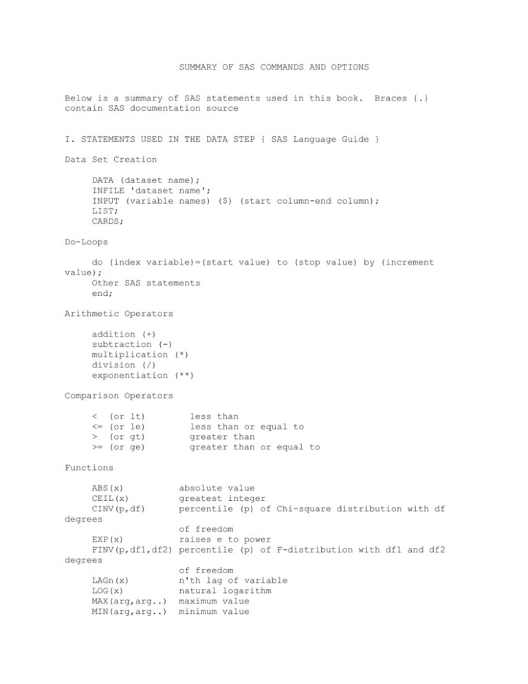
SUMMARY OF SAS COMMANDS AND OPTIONS
Below is a summary of SAS statements used in this book.
contain SAS documentation source
Braces {.}
I. STATEMENTS USED IN THE DATA STEP { SAS Language Guide }
Data Set Creation
DATA (dataset name);
INFILE 'dataset name';
INPUT (variable names) ($) (start column-end column);
LIST;
CARDS;
Do-Loops
do (index variable)=(start value) to (stop value) by (increment
value);
Other SAS statements
end;
Arithmetic Operators
addition (+)
subtraction (-)
multiplication (*)
division (/)
exponentiation (**)
Comparison Operators
<
<=
>
>=
(or
(or
(or
(or
lt)
le)
gt)
ge)
less than
less than or equal to
greater than
greater than or equal to
Functions
ABS(x)
CEIL(x)
CINV(p,df)
degrees
absolute value
greatest integer
percentile (p) of Chi-square distribution with df
of freedom
EXP(x)
raises e to power
FINV(p,df1,df2) percentile (p) of F-distribution with df1 and df2
degrees
of freedom
LAGn(x)
n'th lag of variable
LOG(x)
natural logarithm
MAX(arg,arg..) maximum value
MIN(arg,arg..) minimum value
NORMAL(seed)
PROBCHI(x,df)
PROBIT(x)
PROBNORM(x)
PROBT(x,df)
RANNOR(seed)
RANUNI(seed)
SQRT(x)
TINV(p,df)
UNIFORM(seed)
standard normal random number
CDF of Chi-square random variable with df degrees of
freedom
inverse function of N(0,1) CDF
CDF of N(0,1) random variable
CDF of t-distribution with df degrees of freedom
standard normal random number
uniform random number in [0,1] interval
square root
percentile (p) of t-distribution with df degrees of
freedom
uniform random number in [0,1] interval
Other statements and useful tools
DELETE
deletes observation
SUM statement
variable + expression;
IF-THEN statement
if expression then statement;
IF-THEN; ELSE; statement
if expression then statement;
else expression;
KEEP statement
keep variable1 variable2;
MERGE statement
merge dataset1 dataset2;
_N_ variable
_N_ is observation number
SET statement
set dataset1 dataset2;
SUBSETTING IF statement
if expression;
TITLE statement
title 'descriptive title here';
. (PERIOD)
denotes missing value
II.
STATEMENTS USED IN THE PROC STEP
Print a data set { SAS Procedures Guide }
PROC PRINT (DATA=dataset name);
TITLE 'descriptive title';
VAR (variable names);
RUN;
Sort a data set { SAS Procedures Guide }
PROC SORT (DATA=dataset name);
BY (variable name);
Summary Statistics { SAS Procedures Guide }
PROC MEANS options;
options include:
n
number of observations
mean
mean
min
minimum value
max
maxiumum value
range
range
sum
sum
var
variance
std
sample standard deviation
stderr standard error of the estimate
uss
uncorrected sum of squares
css
corrected sum of squares
t
t-value for mean=0
prt
p-value for "t" test
VAR variables;
OUTPUT OUT='dataset name' MEAN=(variable names) VAR=(variable names)
...;
or
PROC UNIVARIATE options;
options include:
n
number of observations
mean
mean
min
minimum value
max
maxiumum value
range
range
sum
sum
var
variance
std
sample standard deviation
median median
mode
mode
VAR variables;
OUTPUT OUT='dataset name' MEAN=(variable names) VAR=(variable names)
...;
Correlation { SAS Procedures Guide }
PROC CORR;
VAR(variable names);
Frequency Diagrams { SAS Procedures Guide }
PROC CHART;
VBAR (variable name)/options;
HBAR (variable name)/options;
Rough plots { SAS Procedures Guide }
PROC PLOT;
PLOT (Y variable name)*(X variable name) ....;
Linear Regression { SAS/STAT Users' Guide }
PROC REG options;
MODEL dependent = independent/ options;
model options include:
covb
clm
cli
acov
noint
dw
print Cov(b)
print confidence interval for E[y]
print confidence interval for y
heteroskedasticity consistent cov(b)
no intercept in model
Durbin-Watson test
OUTPUT OUT=SASdataset PREDICTED=varname RESIDUAL=varname ...;
Other variables that can be output include:
L95=varname
U95=varname
STDI=varname
lower bound of 95% prediction interval
upper bound of 95% prediction interval
standard error of forecast
WEIGHT varname;
TEST SAS expressions;
RESTRICT SAS expressions;
Systems of Linear Equations { SAS/ETS User's Guide }
PROC SYSLIN options;
PROC SYSLIN options include:
sur
vardef=n
Seemingly Unrelated Regressions
compute variances with no degrees
2sls
freedom correction
two stage least squares
of
ENDOGENOUS variables;
INSTRUMENTS variables;
IDENTITY equation;
MODEL dependent = independent variables;
STEST SAS expressions;
SRESTRICT SAS expressions;
Autoregessive Models { SAS/ETS User's Guide }
PROC AUTOREG options OUTEST=SASdataset;
Model dependent variable = independent variables/options;
options include:
NLAG=n
order of autoregressive model
METHOD=options
ml=maximum likelihood uls=nonlinear least
squares
CONVERGE=n
convergence tolerance
DW=n
Durbin-Watson statistic for order n=1,2,3 or
4
DWPROB
p-value of Durbin-Watson test
LAGDEP=varname
produces Durbin's h-statistic for
autocorrelation
in the presence of a lagged dependent
variable
LAGDEP
produces Durbin's t-statistic for
autocorrelation
in the presence of a lagged dependent
variable
Output out=SASdataset options;
PREDICTED=varname prediction corrected for autocorrelation
PREDICTEDM=varname prediction of mean value
LCL=varname
lower bound of 95% interval for PREDICTED
value
UCL=varname
upper bound of 95% interval for PREDICTED
RESIDUALM=varname
RESIDUAL=varname
residual from prediction of mean value
residual from PREDICTED value
value
Pooling Time-Series and Cross-Sectional Data
}
{ SAS/ETS User's Guide
PROC TSCSREG TS=t CS=n FULLER;
MODEL dependent = independent variables;
or
PROC MIXED;
{ SAS/STAT User's Guide }
CLASS ind time;
identify cross-section
an time-series variables
MODEL dependent = independent/s;
the "s" option prints slopes
RANDOM ind time;
identify which effects are
random
Systems of Nonlinear Equations { SAS/ETS User's Guide }
PROC MODEL;
PARAMETERS parameter names;
program statements
ENDOGENOUS varnames;
INSTRUMENTS varnames;
FIT equations/options;
FIT statment options include:
itsur
it2sls
ols
sur
iterative sur
iterative 2sls
ols (default)
seemingly unrelated regressions
Time-Series Analysis { SAS/ETS User's Guide }
PROC ARIMA;
IDENTIFY VAR=varname(d) NLAG=n;
variable
produces diagnostics for
differenced d times based on n
lags
ESTIMATE P=p Q=q METHOD=options;
FORECAST LEAD=n;
estimate ARIMA(p,d,q)
generate forecasts up to period
T+n
%DFTEST(SASdataset,variable[,options]);
This is a SAS macro that
performs the Dickey-
Fuller
unit root test.
Required arguments are:
the SAS dataset name
variable name.
Options include:
AR=n
DIF=(n)
the number of additional AR terms to
include. Default=3
the degree of differencing to be
DLAG=n
to the series.
specifies the lag to be tested for
OUT=datasetname
OUTSTAT=datasetname
unit root. n=1,2,4 or 12. Default=1.
writes residuals to output dataset.
writes test statistic, estimates, etc
applied
the
to
output dataset.
The macro does not
print
TREND=n
results, so this is necessary to view
results
specifies the degree of deterministic
trend included. n=0 for no trend, n=1
for
intercept, n=2 for intercept and time
trend.
Default=1.
Polynomial Distributed Lags { SAS/ETS User's Guide }
PROC PDLREG options;
MODEL dependent = variable(n,pmax,pmin,constraint);
where
n=lag length
pmax=degree of polynomial
pmin=minimum degree of polynomial
constraint=FIRST, LAST, or BOTH
FIRST imposes head constraint b(-1)=0
LAST imposes tail constraint b(n+1)=0
BOTH imposes both head and tail constraint
Nonlinear Least Squares Regression { SAS/STAT User's Guide }
PROC NLIN METHOD=options;
MODEL dependent = expression;
PARMS parameter=value...;
other program statements
DER.parameter = expression;
Discrete Dependent Variables { SAS/STAT User's Guide }
PROC PROBIT options;
CLASS variables;
MODEL response = variables/D=(normal or logistic) options;
or
PROC LOGISTIC options;
MODEL response = variables/options;