Shortest Paths with Dynamic Programming: Bellman-Ford Algorithm
CMPSC 465 – Kleinberg/Tardos 6.8, CLRS 24.1
I. Problem Statement
Recall the shortest paths problem.:
 One input is a weighted graph, G.
 We’ll have a weight function w: E(G)  R, where w(e) is the weight of edge e.
 We also need a source vertex s and a destination t.
 The problem is to find the shortest directed path from s to t.
 The weight of path p = (v0, v1, …, vn) is given by
k
 w(v
i1
,vi )
i1
Earlier, we solved this problem with Dijkstra’s algorithm, which had the limitation that all edge weights had to be
nonnegative. Now, we’ll remove that restriction.
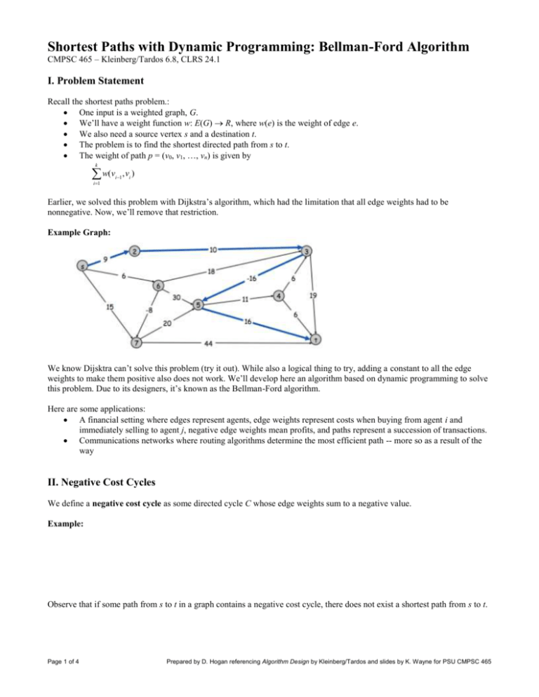
Example Graph:
We know Dijsktra can’t solve this problem (try it out). While also a logical thing to try, adding a constant to all the edge
weights to make them positive also does not work. We’ll develop here an algorithm based on dynamic programming to solve
this problem. Due to its designers, it’s known as the Bellman-Ford algorithm.
Here are some applications:
 A financial setting where edges represent agents, edge weights represent costs when buying from agent i and
immediately selling to agent j, negative edge weights mean profits, and paths represent a succession of transactions.
 Communications networks where routing algorithms determine the most efficient path -- more so as a result of the
way
II. Negative Cost Cycles
We define a negative cost cycle as some directed cycle C whose edge weights sum to a negative value.
Example:
Observe that if some path from s to t in a graph contains a negative cost cycle, there does not exist a shortest path from s to t.
Page 1 of 4
Prepared by D. Hogan referencing Algorithm Design by Kleinberg/Tardos and slides by K. Wayne for PSU CMPSC 465
Theorem: If G has no negative cycles, then for all s, t V(G), there is a shortest path from s to t that is simple.
Proof:
Let G be a graph with no negative cycles and let s, t V(G).
Every cycle has nonneg cost  shortest path P from s to t with fewest number of edges does not repeat any vertex v  V(G).
If P did repeat a vertex v, we could remove the part of P between consecutive visits and get a path with no greater cost and
fewer edges.
Hence a shortest path from s to t must be simple.
Note, then, that we have the precondition that our input graph in which to find shortest paths may not contain negative cost
cycles.
III. Building an Algorithm for Shortest Path Lengths
Let’s further define our problem by saying we are trying to find the shortest path from _____ to ______. v to t
Consider a visualization of such a path:
draw graph from top of p. 293
We’ll “hardcode” the destination and constrain the problem by the number of edges allowed, and have two variables in
subproblems:
 The number of edges allowed in a shortest path
 The source vertex (see illustration above)
As before, we’ll define an OPT measure:
OPT(i, v) =
There are two cases to consider:
 Case where P uses at most i - 1 edges

Case where P uses exactly i edges
Thus, we define OPT(i, v) as follows:
Page 2 of 4
Prepared by D. Hogan referencing Algorithm Design by Kleinberg/Tardos and slides by K. Wayne for PSU CMPSC 465
We can compute the length of the shortest path from v to t in graph G using OPT(|E(G)|-1, v).
[Note that KT seems to be using n for |E(G)|. I’ll always make this explicit for you.]
So, we get the following algorithm for computing the length of shortest paths in a graph G to some vertex t  V(G):
SHORTEST-PATH-LENGTHS(G, t)
M[0, t] = 0
for each vertex v  V(G) – {t}
{
M[0, v] = ∞
}
for i = 1 to |V(G)| - 1
{
for each vertex v  V(G)
{
M[i, v] = M[i-1, v]
}
for each edge (v, u)  E(G)
{
M[i, v] = min( M[i, v], M[i-1, u] + w(v, u) )
}
}
The running time of this algorithm is O( |V(G)| |E(G)| ).
Example: Build the table that results from the above algorithm using the following graph G:
Page 3 of 4
Prepared by D. Hogan referencing Algorithm Design by Kleinberg/Tardos and slides by K. Wayne for PSU CMPSC 465
IV. Finding Shortest Paths
We can change the algorithm to allow us to recover the shortest paths themselves:
 Have each node v maintain the first node (after itself) on its path to the destination t, denoted by first[v].
 We update the value of first[v] every time the distance from v to t is updated.
Here’s an update
SHORTEST-PATH-LENGTHS(G, t)
M[0, t] = 0
first[t] = NIL
for each vertex v  V(G) – {t}
{
M[0, v] = ∞
first[v] = NIL
}
for i = 1 to |V(G)| - 1
{
for each vertex v  V(G)
{
M[i, v] = M[i-1, v]
}
for each edge (v, u)  E(G)
{
if M[i-1, u] + w(v, u) < M[i, v]
{
M[i, v] = M[i-1, u] + w(v, u)
first[v] = u
}
}
}
Problem: Make a trace table illustratin how first changes throughout the execution of this algorithm for the last example.
Problem: What is the shortest path from e to t? What is the shortest path from a to t?
We can also improve the algorithm’s performance by maintaining only one array M[v] of the shortest paths from v to t we
have found so far.
Homework: Try Bellman-Ford on the same graphs you used for the Dijsktra’s algorithm homework. Do CLRS Exercise
24.1-1, but presenting it as we did here, not using CLRS’s flavor of the algorithm.
Page 4 of 4
Prepared by D. Hogan referencing Algorithm Design by Kleinberg/Tardos and slides by K. Wayne for PSU CMPSC 465