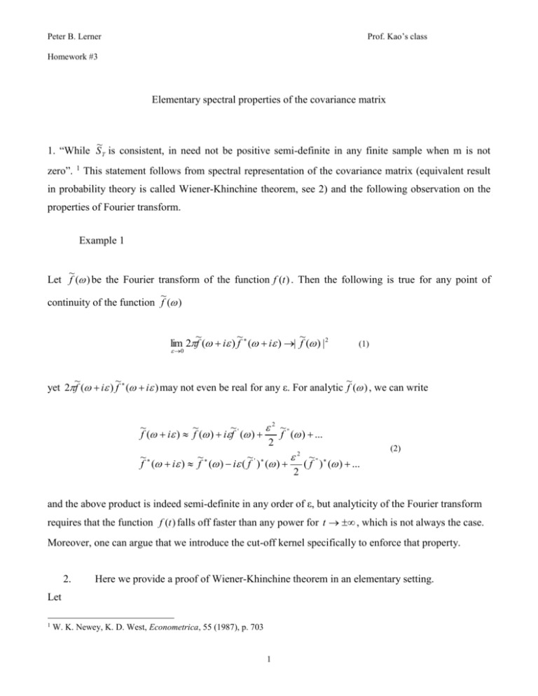
Prof. Kao’s class
Peter B. Lerner
Homework #3
Elementary spectral properties of the covariance matrix
~
1. “While S T is consistent, in need not be positive semi-definite in any finite sample when m is not
zero”. 1 This statement follows from spectral representation of the covariance matrix (equivalent result
in probability theory is called Wiener-Khinchine theorem, see 2) and the following observation on the
properties of Fourier transform.
Example 1
~
Let f ( ) be the Fourier transform of the function f (t ) . Then the following is true for any point of
~
continuity of the function f ( )
~
~
~
lim 2f (  i ) f  (  i ) | f ( ) | 2
 0
(1)
~
~
~
yet 2f (  i ) f  (  i ) may not even be real for any ε. For analytic f ( ) , we can write
~
~
~
 2 ~"
f (  i )  f ( )  if ' ( ) 
f ( )  ...
2
~
~
~' 
 2 ~" 
f (  i )  f ( )  i ( f ) ( ) 
( f ) ( )  ...
2
(2)
and the above product is indeed semi-definite in any order of ε, but analyticity of the Fourier transform
requires that the function f (t ) falls off faster than any power for t   , which is not always the case.
Moreover, one can argue that we introduce the cut-off kernel specifically to enforce that property.
2.
Here we provide a proof of Wiener-Khinchine theorem in an elementary setting.
Let
1
W. K. Newey, K. D. West, Econometrica, 55 (1987), p. 703
1
Prof. Kao’s class
Peter B. Lerner
Homework #3
ht 
 
h e 


i t
(3)
 
Then
j 
 E (ht ht  j ) 
j  

j 
j     
  
j  
 E (h h  )e i t i (t  j ) 
    
j  
   | h |
j   j   
2
e
 i ( j  j  )
 lim
 
   E (h h )e
j  
 | h |  e

2
N 
 
N
j     
 
    
2
ij
N

i (   ) t ij

sin 2 ( N )
 lim  | h | 2
 2 | h0 | 2
2
N 
sin
(

)
  
 
(4)
Third equality sign is the consequence of definition Eq. (3), in the fourth equality we changed an order
of summation and the last equality sign is the result of convergence of sinusoidal-square (Völler) kernel
to the 2 ( ) . This reasoning is not strict but each step can be justified by rigorous estimates.
3.
We expand the variation of the sum of random variables:
m m
 m
 m
Var   ht  j    Var (ht  j )  2 Cov(ht ht  j ) 
j 1 t 1
 j 1
 j 1
m
 E (h j h Tj )  2
j 1
m

m j
m
 E (ht ht  j )  E (h j h Tj ) 
j   m , t 1
j 0
j 1
 (m  j ) E (h h
m
j  m,
j 0
t
T
t j

)  (m  j ) E (ht htT j ) 
(5)
j m
j m
 | j |
T
T
(
m

|
j
|)
E
(
h
h
)

m
1 
E (ht ht  j )


t t j
m 
j  m
j  m 
We can approximate expectation in the last equation by its sample average (Newey and West, Theorem
1).
4. Repeating the argument of the previous paragraph:
j m
 w( j, m)(
j  m
5.
 m

1 T


h
h
)

Var

t t j
sample   ht  j   0 (6)
T t 1
j

1


We have AR(1) process:
2
Prof. Kao’s class
Peter B. Lerner
Homework #3
ht  ht 1   t
(7)
Expansion of the ht provides:
ht   t   t 1   2  t  2  ...(a )
ht  j   t  j    jt 1   2  t  j  2  ...(b)
(8)
Taking variances of both sides of Eq. (8a) and using the i.i.d. property of  t , t ,Var ( t )   2 we
obtain:
Var[ht ]   2   2 2   4 2  ... 
 2
1  2
(9)
For computation of the covariance we notice, that, because of i.i.d. property, series under the expectation
sign begin with the j-th term in regression (8a) and the first term in regression (8b) and
E[ht ht  j ] 

j
 E[  j  t  j  t  j   j 1 t  j 1 t  j 1  ...], j  0  2
,j0
  (1   )

0
0, j  0

j 
j
1
  2
(1   ) 2
j  0 (1   )
j 
 E[ht ht  j ]   2 
j 0
(10)
(11)
Q.E.D.
6. Mixing is a property of random processes, which is weaker than ergodicity but is used
essentially for the same purpose: namely to assure interchangeability between a limit sign and
probability measure. This allows proofs of uniform convergence in the law of large numbers and CLT.
3
Prof. Kao’s class
Peter B. Lerner
Homework #3
There are many non-equivalent definitions of mixing. The naïve idea of mixing is the following2:
consider an shift operator of the random process ξ(t):
S u (t )   (t  u )
Then, mixing means that for t   the points ω of the set StA1 are uniformly distributed over the entire
space Ω, in the sense that for any set in this space, the points ω of StA1 have a measure, which is
proportional to the measure of this set:
lim P( S t A1 )  A2   P( A1 ) P( A2 )
t  
(12)
This property is called “uniform mixing”.
Formal definitions for the most popular types of mixing provided in (Zhenguan, Chuanzhong,
1996) are listed below.3
First, one defines the distance between two subfields A and B of algebra F in one of the
following fashions:
 ( A, B)  sup | P( AB)  P( A) P( B) |
(13)
A, B
 ( A, B)  sup
| E ( AB)  E ( A) E ( B) |
A, B
(14)
VarAVarB
 ( A, B)  sup | P( B | A)  P( B) |
(15)
A, B
and
Fab   ( X i , a  i  b)
Then α- (respectively (ρ, φ))-mixing means that
2
3
Yu. V. Prokhorov, Ya. A. Rozanov, Probability Theory.
Lin Zhenguan, Lu Chuanzhong, Limit Theory for Mixing Dependent Random Variables, (Kluwer, Dordrecht, 1996).
4
Prof. Kao’s class
Peter B. Lerner
Homework #3
sup  ( F1k , Fn k )  0, n  
(16)
k
Mixing property assures that serial correlations between two random processes decrease with time. This
property is important for convergence as one can observe from the following example. 4
Example 2
We estimate the coefficient  n for two scalar processes X t , Z t and E ( X t2 )  1 :
n
 n  n 1  E ( X t Z t )
(17)
t 1
Suppose a sequence for estimation of X t , Z t begins with:
1,3,1,1,3,3,1,1,1,1,...
and repeats indefinitely. Then the coefficient  n will oscillate between 1.5 and 2 no matter how long the
sample is. This example illustrates that the mixing sequence is the sequence, which sweeps the
probability space more or less uniformly.
In their Theorem 2, Condition (iii), Newey and West assume mixing sequences  (l ) ~ O(l   ) ,
 (l ) ~ O(l  ) where   2r /( 2r  1) , r  1 . Otherwise, there will be no assurance that the bandwidth will
have appropriate growth rate. In particular, inequality of Eq. (11), Newey and West can hold only if
m(T) grows slower than T1/4.
4
Domowitz and White. Journal of Economics, 20 (1982) 35-58.
5