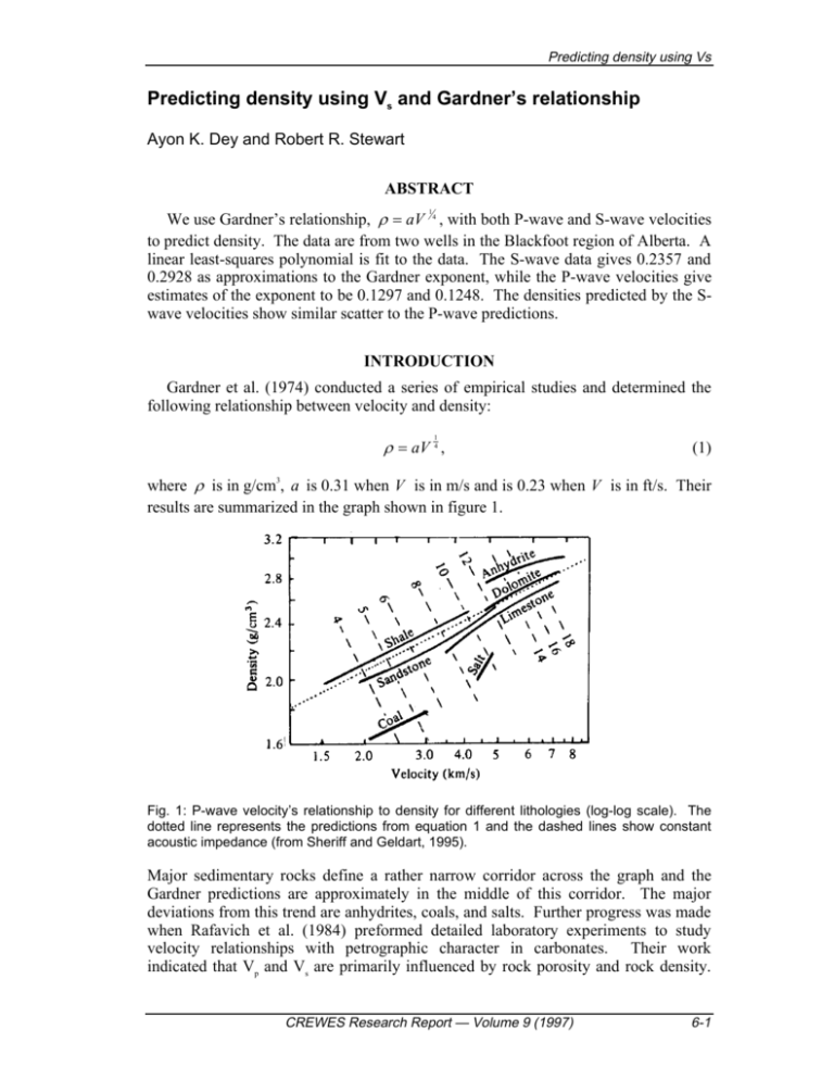
Predicting density using Vs
Predicting density using Vs and Gardner’s relationship
Ayon K. Dey and Robert R. Stewart
ABSTRACT
We use Gardner’s relationship, U aV 4 , with both P-wave and S-wave velocities
to predict density. The data are from two wells in the Blackfoot region of Alberta. A
linear least-squares polynomial is fit to the data. The S-wave data gives 0.2357 and
0.2928 as approximations to the Gardner exponent, while the P-wave velocities give
estimates of the exponent to be 0.1297 and 0.1248. The densities predicted by the Swave velocities show similar scatter to the P-wave predictions.
1
INTRODUCTION
Gardner et al. (1974) conducted a series of empirical studies and determined the
following relationship between velocity and density:
U
1
aV 4 ,
(1)
where U is in g/cm3, a is 0.31 when V is in m/s and is 0.23 when V is in ft/s. Their
results are summarized in the graph shown in figure 1.
Fig. 1: P-wave velocity’s relationship to density for different lithologies (log-log scale). The
dotted line represents the predictions from equation 1 and the dashed lines show constant
acoustic impedance (from Sheriff and Geldart, 1995).
Major sedimentary rocks define a rather narrow corridor across the graph and the
Gardner predictions are approximately in the middle of this corridor. The major
deviations from this trend are anhydrites, coals, and salts. Further progress was made
when Rafavich et al. (1984) preformed detailed laboratory experiments to study
velocity relationships with petrographic character in carbonates. Their work
indicated that Vp and Vs are primarily influenced by rock porosity and rock density.
CREWES Research Report — Volume 9 (1997)
6-1
Dey and Stewart
Lithology, itself, appeared to have only a small influence as did pore shape and
interstitial fluid.
GEOLOGY OF THE REGION
The log data studied in this report are taken from two wells within the Blackfoot
field located near Strathmore, Alberta, in Township 23, Range 23, west of the 4th
meridian. Miller et al. (1995) discuss the initial interpretation of this area’s geology.
Figure 2 shows the stratigraphy near the zone of interest.
Fig. 2: Stratigraphic sequence near the zone of interest (from Miller et al., 1995).
6-2
CREWES Research Report — Volume 9 (1997)
Predicting density using Vs
Table 1: Major geological formation units near zone of interest (from Potter et al., 1996).
ABBREVIATION
FORMATION NAME
2WS
Second White Speckled Shale
BFS
Base of Fish Scales Zone
VIKING
Viking
MANN
Blairmore-Upper Mannville
COAL 1
1 Coal Layer
COAL 2
2 Coal Layer
COAL 3
3 Coal Layer
GLCTOP
Glauconitic Channel Top
LITHCH
Lithic Channel
GLCSS
Glauconitic Channel Porous Sandstone
OST
Ostracod
SUNB
Sunburst
DET
Detrital
MISS
Shunda-Mississippian
st
nd
rd
RESULTS
Tables 2 and 3, modified from Potter et al. (1996), show parameters that are taken
from the well log data. This study uses the 12-16 and 9-17 wells from the study area
because they have dipole sonics over the interest zone, as well as the complete array
of conventional logs. These logs are blocked across the lithological units in Table 1
using MATLAB’s LOGEDIT algorithm with the mean value between the formations
used for the blocking. Tables 2 and 3 show a depth value that corresponds to the top
of the formation and its interval width.
CREWES Research Report — Volume 9 (1997)
6-3
Dey and Stewart
Table 2: Log data for various horizons from the 12-16 well (modified from Potter et al., 1996).
UNIT
DEPTH(m)
Vp(m/s)
Vs(m/s)
U (kg/m3)
Above
1229
3562
1837
2512
2WS
1241
3557
1819
2485
BFS
1328
3303
1520
2390
VIKING
1353
3865
2008
2516
MANN
1445
3987
2018
2525
COAL 1
1519
3485
1683
2256
COAL 2
1525
4121
2120
2472
COAL 3
1538
4071
2103
2516
GLCTOP
1566
3999
2113
2558
GLCSS
1586
4062
2297
2493
DET
1595
4458
2339
2571
MISS
1611
5897
3063
2690
Table 3: Log data for various horizons from the 9-17 well (modified from Potter et al., 1996).
6-4
UNIT
DEPTH(m)
Vp(m/s)
Vs(m/s)
U (kg/m3)
Above
1440
3597
1865
2547
MANN
1450
3862
2011
2528
COAL 1
1526
3416
1659
2305
COAL 2
1532
3971
1996
2508
COAL 3
1545
3890
2031
2561
SUNB
1593
4072
2122
2550
DET
1606
4170
2184
2538
MISS
1637
5061
2421
2669
CREWES Research Report — Volume 9 (1997)
Predicting density using Vs
Below are Vp versus U plots and Vs versus U plots for two well logs from the
Blackfoot region of Alberta. The data being cross-plotted are the densities, P-wave
velocities, and S-wave velocities from the 12-16 and 9-17 well logs. If the data is
plotted in log-log style, then the slope of a best-fit line to this data is an
approximation to the Gardner exponent. This is shown by the following equation:
log e ( U )
1
log e (V ) log e (a ) .
4
(2)
Equation 2 also tells us that the y-intercept of the line, log e (a ) , is the natural
logarithm of an estimate to the Gardner coefficient. The line shown on these plots is
the best-fit (in a least-squares sense) linear polynomial to the given data.
Fig. 3: Vp versus U log-log plot with linear curve fitting for the 12-16 well.
CREWES Research Report — Volume 9 (1997)
6-5
Dey and Stewart
Fig. 4: Vs versus U log-log plot with linear curve fitting for the 12-16 well.
Fig. 5: Vp versus U log-log plot with linear curve fitting for the 9-17 well.
6-6
CREWES Research Report — Volume 9 (1997)
Predicting density using Vs
Fig. 6: Vs versus U log-log plot with linear curve fitting for the 9-17 well.
What we see from all of these four plots is that the conventional method, i.e. using Vp,
of treating Gardner’s relationship seems to give a poorer estimation of the Gardner
exponent than if we use shear wave velocity. For the 12-16 well, the P-wave velocity
approximation to the Gardner exponent has an absolute deviation from the expected
value, 0.24, of 0.1103. In the meantime, the S-wave velocity approximation has only
a 0.0043 absolute deviation from the expected value. When considering the 9-17
well, it is seen that the P-wave estimate deviates from the norm by 0.1152 and the Swave estimate only fluctuates by 0.0528. While it is unconventional to use Vs in
Gardner’s relationship, these preliminary results seem to encourage its use. As a
means to understand the goodness of this fit to the data, we use the MATLAB
functions std and cov. These functions give us values for the standard deviation, V ,
the variance, V 2 , and the correlation coefficient, cc , respectively. With these values,
we can evaluate the scatter of the data. One should note that the std function
normalizes by (n-1), where n is the number of samples in the sequence, and this
makes cov the best estimate of the variance in the data. Table 4 summarizes these
statistical results.
CREWES Research Report — Volume 9 (1997)
6-7
Dey and Stewart
Table 4: Statistical analysis values for density models.
Vp Density Model
12-16 Well:
9-17 Well:
Vs Density Model
V
0.0869
V
0.0907
V2
0.0076
V2
0.0082
V
0.0674
V
0.0653
V2
0.0045
V2
0.0043
These statistical results seem to strengthen the argument for using shear wave
velocities to predict density. We see that for the 12-16 well, the standard deviation
and variance for the Vs model are quite similar to the values for the Vp model. The 917 well results seem to offer better statistics in that both the standard deviation and
the variance are lower for the Vs model.
CONCLUSIONS AND FURTHER DIRECTIONS
A preliminary conclusion that we draw from this investigation is that using S-wave
velocities to predict density with Gardner’s relationship seems to give a better
approximation to the Gardner exponent. In addition, the statistical analysis seems to
suggest that the shear wave model has standard deviations and variances that are
similar to, or possibly better than, those of the P-wave model. While these results are
very encouraging, there are still some significant issues to address. First, we must
test the use of Vs in Gardner’s relationship with well log data from other areas.
Namely, we wish to test this hypothesis with data from regions that have a lithology
that varies from that which is seen in the Blackfoot region. In addition to this, we
must also extrapolate these best fit lines back to the y-axis. This will give us a value,
when converted under logarithmic inversion, that estimates the Gardner coefficient.
Only when this component can also be shown to have a better approximation with Vs
can we recommend the use of Vs as routine practice when considering density
predictions with Gardner’s relationship. As a final path of investigation, we hope to
look at Lindseth’s relationship, UE aE k , and see how its estimates of density
compare to approximations given by Gardner’s relation.
REFERENCES
Gardner, G.H.F., Gardner, L.W., and Gregory, A.R., 1974, Formation velocity and density – the
diagnostic basics for stratigraphic traps: Geophysics, 39, 770-780.
6-8
CREWES Research Report — Volume 9 (1997)
Predicting density using Vs
Kithas, B.A., 1976, Lithology, gas detection, and rock properties from acoustic logging systems:
th
Society of Professional Well Log Analysts 17 Annual Symposium.
Miller, S.L.M., 1992, Well log analysis of Vp and Vs in carbonates: CREWES Research Report,
volume 4.
Potter, C.C., Miller, S.L.M., and Margrave, G.F., 1996, Formation elastic parameters and synthetic P-P
and P-S seismograms for the Blackfoot field: CREWES Research Report, volume 8.
Rafavich, F., Kendall, C.H.St.C., and Todd, T.P., 1984, The relationship between acoustic properties
and the petrographic character of carbonate rocks: Geophysics, 49, 1622-1636.
Sheriff, R.E., and Geldart, L.P., 1995, Exploration Seismology, Second Edition: Cambridge University
Press, New York, N.Y., U.S.A.
CREWES Research Report — Volume 9 (1997)
6-9