AP* Chemistry
CHEAT SHEET FOR KINETICS
Integrated Rate Law
FOR THE TI-83+ or 84+ CALCULATOR NOVICE:
BEFORE ENTERING LISTS AND GRAPHING:
• First set up housekeeping! Press É‘ to clear your “home” screen.
Next, let us clear your lists & get “Diagnostics On”
o Press y à and your screen will look like this:
o Press ¶ to select “Clear all lists”. Hit Í to execute the command.
o It will say “Done” if you were successful and your screen will look
like this:
o Next, we will set the calculator to float the decimal point. Press z
and use your arrow keys to place your cursor on “Float”. If it is dark,
it’s fine. If it isn’t then hit Í once the
“Float” is flashing to turn it on. It is on if it is
dark.
Press yz to quit this screen.
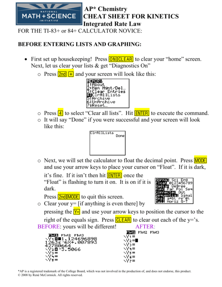
o Clear your y= [if anything is even there] by
pressing the o and use your arrow keys to position the cursor to the
right of the equals sign. Press ‘ to clear out each of the y=’s.
BEFORE: yours will be different!
AFTER:
*AP is a registered trademark of the College Board, which was not involved in the production of, and does not endorse, this product.
© 2008 by René McCormick. All rights reserved.
Just FYI: if the equals sign is dark, the equation will be graphed. You
can leave the equations and turn off the graphing of the function by
positioning your cursor over the = and pressing ENTER.
So far, so good—on to the last bit of housekeeping.
o Press yÊ to get to catalogue. Notice the Ø in the upper right
corner—it means the “alpha lock” is on and you can hit the — key
[located 3 buttons down from the yellow y key] to get to the D’s.
We want to turn “Diagnostics On”.
o Press † unitl your cursor is to the left of
“Diagnostics On.”. Press ÍÍ
{no, this is NOT a typo! once pastes the command and the second
executes it!} Your
screen will look like this:
• This has set up your calculator with clear lists and the ability to give us an
“r” when we run a linear regression. Some kid will need to know how to do
this before you finish the lesson!
TO ENTER DATA INTO LISTS
• Press …. Your screen will look like this:
• Press À to edit and your screen changes to
this:
• Let’s enter the data from Exercise 12.2 in your
notes. Time is the independent variable and goes into L1 (to be plotted on
the x-axis). Hit Í after each number and the cursor moves down the
lists. Concentration in L2.
[N2O5]
0.1000
0.0707
0.0500
0.0250
0.0125
0.00625
Time (s)
0
50
100
200
300
400
• If you mess up, just use your arrow keys to
navigate to the goof and type over it! When all
the data is entered, your screen will look like this:
Cheat Sheet for Kinetics, Integrated Rate Law
2
TO UTILIZE THE CALCULATOR AND INTEGRATED RATE LAW
You can determine the order of a reactant and k in a flash using the calculator.
ALSO, remember, the equation of a straight line is in y = ax + b format for the
TI calculator. Once you have this equation in y= AND you can graph the
equation, you use it to solve for time! Much faster than the way you and I
learned to do this!!
The notes say:
Using the graphing calculator: Set up your calculator so that (the y-list is alphabetical!)
L1 Λ time (x variable throughout!)
L2 Λ concentration
[A]
L3 Λ ln concentration
ln [A]
L4 Λ reciprocal concentration 1/[A]
Run a linear regression on L1,L2; L1,L3; L1,L4 and see which has the best Ar@
L1 is time and already in there as is L2 which is simply concentration.
• L3 is the “natural log” or ln of concentration. Go to the “tippy top” of L3 by
hitting ~ then }. Next, hit μyÁ which will register at the bottom of
the screen—you don’t need to close the parentheses, just hit Í to
magically transform all the data in L2 into natural logs and plop it into L3. If
successful, your screen will look like this:
If you’re not at the “tippy top” it won’t work!!!!! try again by pressing
… then À and arrowing around to the “tippy top” of the list!
Cheat Sheet for Kinetics, Integrated Rate Law
3
• Press ~ then } to get to the “tippy top” of L4 and press yÁ—Í to
transform L4 into reciprocals of L2. You can only display 3 lists at a time so
note the shift—L1 has “disappeared” from our screen. If successful, your
screen should look like this:
RUNNING A LINEAR REGRESSION
• Press … then ~ to CALC. Your screen
changes to this:
• Press ¶ . This pastes LinReg(ax+b) on your
screen. Next you must tell the calculator where
to get the (x,y) ordered pair. We want
(time,conc.) to start so press yÀ¢yÁ to
paste L1,L2 after the LinReg command. Press
Í. Your screen will look like this:
o At first, you may think the “r”—linear regression correlation
coefficient is great at .9anything, BUT it isn’t. I usually speak of
playing poker at this stage and I’m trying to beat this “hand” so keep
going….
o Press yÍ to get the last command on
the screen. Press | to place the cursor over
L2 and press yÂÍ to convert it to L3.
If successful, your screen looks like this:
Oh, my! Quite a hand! Because you’re the
teacher, keep going…
o Press yÍ to get the last command on
the screen. Press | to place the cursor over
L3 and press y¶Í to convert it to L4.
If successful, your screen looks like this:
Cheat Sheet for Kinetics, Integrated Rate Law
4
• Since L1,L3 was the best “r” value, it is the set we should use to determine
everything else.
Look at the best set of data’s regression statistics again:
Since ln[conc.] vs. time was the most direct relationship [i.e. best “r”, best fitting
straight line] the reaction is first order, so ….
Rate = k[N2O5]
AND…
The k is equal to the absolute value of the slope
Rate = 6.93 x 10 –3 [N2O5]
sec
• Press yÍ repeatedly until you get back to
LinReg(ax+b)L1,L3 Now we paste it into Y=
by…
o Press ¢then  then ~to get to YVARS then Àto get to functions then À
(or whichever Y function you want to place
the regression equation in). Your screen will look like this:
o Press Í once you have the screen above.
o If there is anything before the command it won’t work! Arrow to the
junk in front of the command and use the { key to remove it—don’t
erase your command!
ƒ You won’t notice anything different at
first. To see if it worked, press the o
button and the numbers should have
been lifted from the linear regression
statistics screen and plopped into a y =
ax + b format. Your screen should look
like this:
TO VIEW AND CALCULATE WITH THE REGRESSION GRAPH
• First, we need to set up your Stat Plots. Press
yo to get to Stat Plot. You’ll get this
screen which may have different settings than
mine….we’ll make them match in the next
step.
Cheat Sheet for Kinetics, Integrated Rate Law
5
o Press Í to get into the Plot 1 menu. Whatever is “dark” [TI says
“highlighted”—kids understand dark better!] is ON and you use your
arrow keys to move up and down while using your ENTER button to
make the “dark” stay. You will have to arrow away from your
changes to see if they “took”. To get
the L1 and L3 use yÀand yÂ
Make your screen look like this:
o Press yo again to check that the
other two plots are off—if they aren’t,
hit their number to go into their menu, then use the arrows and
ENTER key to make “OFF” dark.
o Press q® to auto fit the screen and make enemies in the math
department! [Check with the
Algebra II teacher before teaching
pre-AP this shortcut!!]. The graph
magically appears and if you watch,
the linear regression line is drawn
in—my favorite part! Your screen
now looks like this:
• To calculate the ln [concentration] {since this is first order} when you
know the time:
o First, check that the value you want to use for time falls between the
Xmin and Xmax by pressing p. If your value does NOT fit into
that range, change the range using your arrow keys to go up and down
and just type in something that will work for you! Press s to
return to your graph.
Cheat Sheet for Kinetics, Integrated Rate Law
6
o From the screen displaying your graph, press yrÀ to display
an X= at the bottom left corner of the graph screen. Type in your time
value [use 150 s for now] and press Í to display the
corresponding ln[N2O5] in the bottom right corner of the screen. It
will look like this:
WHAT??? A negative concentration?? Oh, I remember…
o If you want the REAL concentration, write down the Y-value you just
solved for and press yz to quit the graph. Press yμ then
the value Ì3.342 thenÍ to get a real concentration of 0.0354 M.
o If you want to keep going, just press s yrÀ to begin
again. If you went out of your window range you get ERR:INVALID
and two choices. If you choose the preferred GOTO, it won’t help—
this time choose QUIT and fix your Xmin and Xmax. Try again!
o Press p, arrow to change your Xmin and/or Xmax values, press
s to return to your graph and repeat the steps by pressing
yrÀ to display an X= at the bottom left corner of the graph
screen. Type in your time value.
HOW DO I GET A TIME IF I’M GIVEN A CONCENTRATION?
To get an X-value (time) when you know a Y-value (remember this one is ln
[conc.]) It’s easiest to first find the ln of the concentration you are using as your
Y-value.
ƒ Press yzto quit the graph and get to the home screen.
Next press μ and the value you want to use. I’ll use 0.0300M
since that’s within our data table yet not in our data table.
ƒ The value is –3.5066. Next I make an equation for this value in
Y=. To do this press o† to Y2 [DON’T overwrite your Y1!].
Type in Ì 3.5066.
Cheat Sheet for Kinetics, Integrated Rate Law
7
ƒ Press s to see that you now have a horizontal line
intersecting your regression line. Next, press
yr·ÍÍÍ. Why three ENTER’s? The
math teachers like to put lots of intersections on the calculator
and the cursor hops from line to line with the arrow keys. Since
we only have 2 lines, the first ENTER selects the first line, the
cursor hops, the second ENTER selects the second line, the
cursor then asks for a “guess”—we don’t have time for that!!—
we want the “answer” so the third ENTER gives us the
intersection value as you see here:
ƒ The time value is therefore, 173.7
seconds. Does that make sense?
Examine the original data table for
enlightenment.
Cheat Sheet for Kinetics, Integrated Rate Law
8