I. Budimir, N. Mrvac, M. Matijević
Utjecaj debljine rešetke kod Munker-Whiteovog efekta
ISSN 1330-3651 (Print), ISSN 1848-6339 (Online)
DOI: 10.17559/TV-20140821220932
THE INFLUENCE OF THE THICKNESS OF THE GRID IN MUNKER-WHITE EFFECT
Ivan Budimir, Nikola Mrvac, Mile Matijević
Original scientific paper
This paper shows the influence of the thickness of the grid on the intensity and assimilation in Munker-White effect. It can be described as the effect of
assimilation of grey rectangular elements into the colour of unbroken lines. They are perceived darker in combination with grey and black lines, and
lighter in white and grey combination. Measured colorimetric differences are shown in CIEDE2000 system. Three polynomial statistical regression
models were created based on the results. Models contain polynomial expressions describing the influence of the grid thickness on the intensity shift of
rectangular objects in Munker-White effect. Models were tested statistically and the analysis of measured parameters shows their statistical
representativeness.
Keywords: assimilation; mathematical model; Munker-White; regression analysis; simultaneous contrast
Utjecaj debljine rešetke kod Munker-Whiteovog efekta
Izvorni znanstveni članak
U radu je opisan utjecaj debljine rešetke na intenzitet simultanog kontrasta i asimilacije kod Munker-Whiteove efekta. Isti možemo opisati kao pojavu
gdje se sivi elementi (pravokutni elementi) asimiliraju s bojom neprekinutih linija, koje se u kombinaciji sa sivo-crnim linijama percipiraju tamnije, a sa
sivo-bijelim linijama svjetlije. Dobivene kolorimetrijske razlike prikazane su u CIEDE2000 sustavu. Na temelju rezultata napravljena su tri polinomijalna
statistička regresijska modela. Modeli sadrže polinomijalne izraze koji opisuju utjecaj debljine rešetke na intenzitet pomaka pojavnosti svjetline
pravokutnih elemenata kod Munker-Whiteovog efekta. Modeli su statistički testirani te je analizom dobivenih parametara pokazano da su statistički
reprezentativni.
Ključne riječi: asimilacija; matematički model; Munker-White; regresijska analiza; simultani kontrast
1
Introduction
While attempting to analyse the psychophysical
visual effect shown in the design of Susan Hirth [1]
Michael White designed in 1979 a brand new black and
white grid structure known as Munker-White illusion [2].
Today it is known as the strongest illusion of whiteness
[4] and it connects psychophysical effect of simultaneous
contrast and assimilation. Simultaneous contrast is the
psychophysical effect which causes the shift of colour
appearance in response to the colour change of the
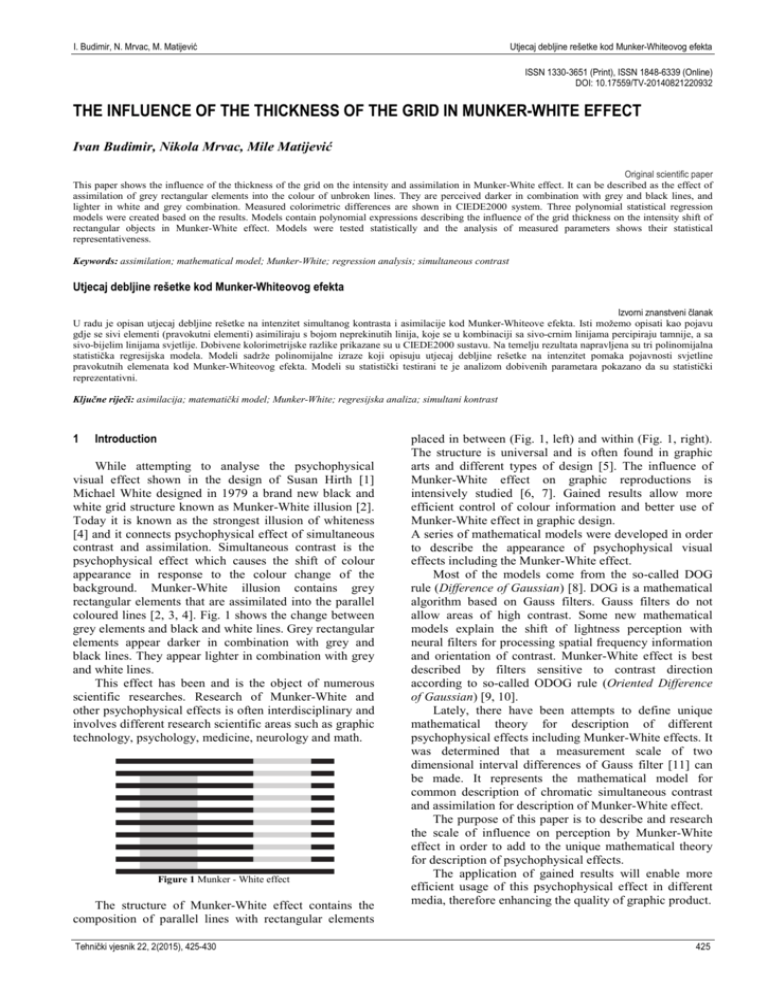
background. Munker-White illusion contains grey
rectangular elements that are assimilated into the parallel
coloured lines [2, 3, 4]. Fig. 1 shows the change between
grey elements and black and white lines. Grey rectangular
elements appear darker in combination with grey and
black lines. They appear lighter in combination with grey
and white lines.
This effect has been and is the object of numerous
scientific researches. Research of Munker-White and
other psychophysical effects is often interdisciplinary and
involves different research scientific areas such as graphic
technology, psychology, medicine, neurology and math.
Figure 1 Munker - White effect
The structure of Munker-White effect contains the
composition of parallel lines with rectangular elements
Tehnički vjesnik 22, 2(2015), 425-430
placed in between (Fig. 1, left) and within (Fig. 1, right).
The structure is universal and is often found in graphic
arts and different types of design [5]. The influence of
Munker-White effect on graphic reproductions is
intensively studied [6, 7]. Gained results allow more
efficient control of colour information and better use of
Munker-White effect in graphic design.
A series of mathematical models were developed in order
to describe the appearance of psychophysical visual
effects including the Munker-White effect.
Most of the models come from the so-called DOG
rule (Difference of Gaussian) [8]. DOG is a mathematical
algorithm based on Gauss filters. Gauss filters do not
allow areas of high contrast. Some new mathematical
models explain the shift of lightness perception with
neural filters for processing spatial frequency information
and orientation of contrast. Munker-White effect is best
described by filters sensitive to contrast direction
according to so-called ODOG rule (Oriented Difference
of Gaussian) [9, 10].
Lately, there have been attempts to define unique
mathematical theory for description of different
psychophysical effects including Munker-White effects. It
was determined that a measurement scale of two
dimensional interval differences of Gauss filter [11] can
be made. It represents the mathematical model for
common description of chromatic simultaneous contrast
and assimilation for description of Munker-White effect.
The purpose of this paper is to describe and research
the scale of influence on perception by Munker-White
effect in order to add to the unique mathematical theory
for description of psychophysical effects.
The application of gained results will enable more
efficient usage of this psychophysical effect in different
media, therefore enhancing the quality of graphic product.
425
The influence of the thickness of the grid in Munker-White effect
I. Budimir, N. Mrvac, M. Matijević
2 Experimental part
2.1 Research description
θ  H
tan   = ,
2 2
Experimental part is composed of instrumental and
visual research.
Spectrophotometric measurement and display of CIE
L*a*b* values are made in instrumental part of the
experiment. Relevant fields were defined with the visual
part of the experiment. The method of binocular
adjustments was used [12].
Deviations in perception caused by certain
manifestation of visual effect are shown as difference of
lightness ΔL00 by applying reference sample from colour
atlas to the sample [7, 14].
Difference in colour ΔE00 and lightness ΔL00 is
calculated with formula [13]:
θ = 2 arctan 
 ΔL'
ΔE00 = 
 k L S L

 ΔC' ab
+ RT 
 kC SC
SL = 1+
2
2
  ΔC' ab
 + 

  kC SC



 ΔH ' ab

 k S
 H H
(
0 ,015 L − 50
(
)
  ΔH ' ab
 +
 k S
  H H
− 0 ,5
20 + L − 50 2 


(1)
,
)2
0 ,5
,
(2)
S C = 1 + 0 ,045C ' ab ,
(3)
S H = 1 + 0 ,015C ' ab T ,
(4)
Where
T = 1 − 0 ,17 cos (h ' ab −30°) + 0 ,24 cos (2h ' ab ) +
+ 0 ,32 cos (3h ' ab +6°) − 0 ,20 cos (4h ' ab −63°),
RT = −sin (2ΔΘ ) RC ,
 h ,

 2d 
(10)
where θ is the viewing angle, H is the test sample size.
Figure 2 Dimensions of Munker - White grid described with x, y and h
2

 +

(9)
(5)
(6)
Table 1 Dimensions of different variants of Munker-White grid in mm
and grid coverage percentage
Nr. of
samples
1
2
3
4
5
6
7
8
9
10
11
x
1
2
3
4
5
6
7
8
8,5
9
10
Grid dimensions
y
h
12
106
11,5
106,5
11,5
107,5
12
108,5
11,5
109
12
110
12
111
12
111
11
111
11
111
11
111
Percentage of
coverage (x/y) / %
8,33
17,39
26,09
33,33
43,49
50,00
58,33
66,67
77,27
81,82
90,91
Test sheet was made in Adobe Photoshop CS5 using
Lab colour space (Fig. 3). It contains test samples and the
appropriate colour atlas.
where
  h ' −275°  2 

 ,
ΔΘ = 30 exp −  ab

25
 
 
 C' 7
RC = 2 7 ab 7
 C ' +25
 ab




(7)
0 ,5
.
(8)
2.2 Design and reproduction of test samples
11 variants of achromatic Munker-White samples
with different grid thickness were made (Fig. 2, Tab. 1)
for the experiment. All the samples are rectangular
elements with the same parameters L = 75,03; a* = 2,63;
b* = −6,88. Values x, y and h are modified for the
experiment.
Dimensions of sample fields were defined in
accordance with standard observing conditions (ISO
3664:2009 which defines observation conditions for
printing industry and professional photography). The
height of test field, viewing angle and test subject distance
were calculated from formula [15]:
Figure 3 Test sheet (test samples and atlas)
426
Technical Gazette 22, 2(2015), 425-430
I. Budimir, N. Mrvac, M. Matijević
Utjecaj debljine rešetke kod Munker-Whiteovog efekta
Reference atlas was made for evaluation of test
samples. Atlas is based on the alteration of perception
attributes within Lab colour model. It contains complete
potential area of perception. Specific fields of atlas have
appropriate CIE L*a*b* values of spectrophotometric
measurements.
Test samples were printed on calibrated printing
machine Canon iX6550. Files were rendered using Adobe
Photoshop CS5. Rendering from Lab colour space to
Canon iX6500 series MP colour profile was done using
perception rendering and Adobe ACE colour engine.
Canon matte photo paper, weight 170 g/m2 was used as
printing substrate. Prior to printing substrate was
conditioned in the room for 48 hours according to
prescribed
standard
environmental
conditions
(temperature of 23 °C and 55 % relative humidity). Test
runs were made at qty. of 10 samples.
2.4 Visual analysis
38 people of mixed population of average age of 20
were used for the visual part of the research. Everyone
passed the Ishihara test prior to testing. Visual evaluation
was performed in controlled ambient conditions (ISO
3664:2009: 10° viewing angle, distance from sample to
test subject 60 cm, natural matte grey surroundings,
artificial lights). Test samples were evaluated under
standard CIR D75 (7500K) lighting.
Visual evaluation was made in accordance with the
method of binocular harmonisation. Test sample and
reference file were in the field of view at the same time.
Every person had to choose a field in the atlas most like
the surface covered by rectangular elements between
black lines (left) and within black lines (right) of the test
sample (Fig. 4).
2.3 Instrumental analysis
X-Rite SpectroEye was used for measuring samples
and reference fields. It measures wavelengths from 380 to
730 nm in increments of 10 (with inner resolution of 3,3
nm). Light source is gaseous wolfram type A. Lighting
geometry is 45°/0°, DIN 5033 with linearisation of
±0,01D.
Each control field in run of 10 copies was measured 5
times after which statistical values were taken in order to
enhance statistical accuracy.
Figure 4 Principle of visual evaluation
Table 2 Mean value, median and standard deviation of L*, a* and b* components of analysed elements (left)
Percentage of
coverage (x/y)
Mean value
%
8,33
70,66
17,39
69,13
26,09
66,77
33,33
67,11
43,49
65,26
50,00
63,99
58,33
63,26
66,67
64,82
77,27
67,00
81,82
70,57
90,91
75,18
L*
Median
70,96
69,35
66,05
66,05
66,05
64,16
64,14
67,72
69,35
72,56
72,56
Std.
deviation
3,37
4,41
4,35
5,47
6,11
7,10
7,95
8,64
6,70
6,63
6,59
a*
Mean value
Median
2,46
2,32
2,11
2,07
1,98
1,90
1,89
1,97
2,16
2,41
2,78
2,51
2,50
2,01
1,89
1,90
1,90
1,90
2,01
2,50
2,50
2,77
Std.
deviation
0,32
0,39
0,42
0,45
0,45
0,50
0,59
0,59
0,53
0,53
0,42
b*
Mean value
Median
−7,82
−7,72
−7,56
−7,46
−7,43
−7,31
−7,27
−7,37
−7,15
−7,64
−7,80
-7,83
−7,83
−7,42
−7,37
−7,32
−7,32
−7,20
−7,41
−7,53
−7,81
−7,83
Std.
deviation
0,34
0,42
0,45
0,36
0,49
0,48
0,61
0,59
2,39
0,36
0,36
Table 3 Mean value, median and standard deviation of L*, a* and b* components of analysed elements (right)
Percentage of
coverage (x/y)
Mean value
%
8,33
81,84
17,39
80,11
26,09
80,04
33,33
80,36
43,49
79,54
50,00
79,17
58,33
79,16
66,67
78,58
77,27
78,23
81,82
78,64
90,91
78,12
3
Results and discussion
Tehnički vjesnik 22, 2(2015), 425-430
L*
Median
81,89
80,83
79,74
79,74
79,74
79,74
80,83
78,54
78,54
78,54
77,98
Std.
deviation
5,35
4,30
4,31
4,47
4,13
4,04
3,91
4,35
4,27
4,93
5,07
a*
Mean value
Median
3,21
3,14
3,13
3,14
3,10
3,12
3,12
3,05
3,03
3,00
2,98
3,29
3,22
3,22
3,22
3,22
3,22
3,22
3,09
3,09
3,09
3,05
Std.
deviation
0,26
0,27
0,27
0,27
0,27
0,24
0,25
0,22
0,23
0,32
0,32
b*
Mean value
Median
−7,85
−7,33
−7,77
−7,80
−7,73
−7,77
−7,79
−7,71
−7,67
−7,73
−7,75
−7,84
−7,81
−7,84
−7,84
−7,82
−7,84
−7,84
−7,79
−7,52
−7,79
−7,82
Std.
deviation
0,36
2,47
0,25
0,27
0,23
0,26
0,22
0,26
0,25
0,28
0,25
Results were statistically analysed with computer
software Statistica 12. Descriptive statistic, correlation
427
The influence of the thickness of the grid in Munker-White effect
I. Budimir, N. Mrvac, M. Matijević
and polynomial regression analysis of the samples were
made.
3.1 Descriptive sample statistic
Tabs. 2 and 3 show descriptive statistical analysis of
psychophysical visual experiment, mean values, medians
and standard deviations of perceived L*, a*, b* values of
analysed elements (Fig. 4, Tab. 1).
Values were calculated with statistical analysis of
results of visual experiment on 38 people.
3.2 Regression analysis of samples
Based on gained results (Tab. 2 and 3) CIEDL00
values were calculated in perceived lightness on
rectangular elements of the grid (Tab. 4) for appropriate
coverage percentage. Colorimetric deviations between
percepted and physical lightness of analysed elements
were calculated (Tab. 4).
Differences were calculated for certain coverage
percentage marked as P.
Table 4 CIEDL00 Colorimetric differences of analysed elements
Value ΔL*2000
Percentage of
(between grid,
coverage P / %
left)
8,33
17,39
26,09
33,33
43,49
50,00
58,33
66,67
77,27
81,82
90,91
−3,27
−4,45
−6,32
−6,05
−7,54
−8,59
−9,2
−7,90
−6,14
−3,34
0,06
Value
ΔL*2000
(within grid,
right)
4,79
3,61
3,56
3,77
3,21
2,95
2,95
2,54
2,3
2,58
2,22
Value
ΔL*2000
(between)
8,05
8,05
9,87
9,81
10,74
11,53
12,13
10,43
8,43
5,92
2,11
Polynomial regression analysis was used to process
available data from Tab. 4. Results are shown in Tabs. 6,
7 and 8.
Correlation analysis of variables ΔL*2000 (between
grid), value ΔL*2000 (within grid) and value ΔL*2000
(between) gave Pearsons correlation coefficients (Tab. 5).
Table 5.Results of correlative analysis of variables ΔL*2000 (between
grid), ΔL*2000 (within grid) i value ΔL*2000 (between) with level of
significance p < 0,05. Table contains the appropriate p-values
Variables
ΔL*2000
(between grid,
left)
ΔL*2000
(within grid,
right)
ΔL*2000
(between)
ΔL*2000
(between
grid, left)
ΔL*2000 (within
grid, right)
ΔL*2000
(between)
1,00
p=.....
0,0129
p=0,970
0,9634
p=0,000
0,0129
p=0,970
1,00
p=.....
0,2564
p=0,447
0,9634
p=0,000
0,2564
p=0,447
1,00
p=.....
Results in Tab. 5 show high negative correlation of
variables ΔL*2000 (between grid) and ΔL*2000 (between)
with Pearson’s correlation coefficients r = −0,9634. This
correlation is statistically significant with level of
significance p = 0,000 < 0,05. Correlations between other
variables are not statistically significant.
3.3 Regression model of colorimetric deviation in lightness
between Munker-White grid
Square regression model gives the dependance of
intensity of lightness shift in regard to the thickness of the
grid for the rectangular elements that are within the
system of parallel lines. Square regression model was
chosen based on the parameters which show high degree
of similarity with the visual research data.
Table 6 Result of regressive analysis of variable ΔL*2000 for rectangular elements between parallel lines (left) in dependance on coverage percentage of
Munker-White grid
N=11
Free coefficient
p
p2
Results of Regression Analysis for Dependent Variable: ΔL*2000, R= 0,93626682, R2=0 ,87659555,
Adjusted R2= 0,84574444, F(2,8)=28,414, p<0,00023, Standard Error of Estimate: 1,0809
b*
Std. Err. of b*
b
Std. Err. of b
t(8)
p-value
0,7703
1,213180
0,63492
0,543209
−3,83773
0,553363
−38,6503
5,572998
−6,93528
0,000120
4,10677
0,553363
40,4074
5,444659
7,42147
0,000075
Determination coefficient R2 = 0,87659555 is very
close to maximal value 1 which shows that the model is
representative. This model can interpret 87,66% of square
errors. Significance of regression is determined with pvalue which for this model is p = 0,00023 < 0,01.
Corrected determination coefficient adjusted R2=
0,84574444 is another indicator of high quality of the
model. The parameter depends on number of liberty
degrees of freedom. Standard error SE = 0,10809 gives an
average deviation of data from regression curve. SE and
p-values of P and P2 are relatively small which shows the
value of the model. P-values are below significance level
of 0,001.
Regression polynomial of second order which gives
the analytical description of dependance of lightness shift
428
ΔL*2000 in dependance on percentage of grid coverage
percentage P was calculated.
ΔL(P) = 0,7703 – 38,6503P + 40,4074P2.
Results show the direction and intensity in lightness
shift (Fig. 5). In almost all cases visual square elements
are perceived as lighter than their measured values.
Largest colorimetric value of −8,4721 is found in grid
coverage of 47,82 %:
{
}
min 0 ,7703 − 38,6503 x + 40 ,4074 x 2 ≈
≈ −8,4721 at x ≈ 0 ,478258.
Technical Gazette 22, 2(2015), 425-430
I. Budimir, N. Mrvac, M. Matijević
Utjecaj debljine rešetke kod Munker-Whiteovog efekta
Colorimetric differences are smaller with very small
and very large coverage percentage.
REGRESSION POLYNOM
95% confidence interval
2
0
Delta L 2000
-2
-4
-6
-8
-10
0,0
0,1
0,2
0,3
0,4
0,5
0,6
0,7
0,8
0,9
1,0
variable P
Figure 5 Graphical representation of regression polynome
3.4 Regression model of colorimetric differences in
ellement within Munker- White grid
Combination of multiple polynome regression models
determined that the data fit best in linear regression
model. It can be determined with high statistical precision
that the difference of colorimetric values dependant on
thickness of the grid is linear.
Determination coefficient of regression model is R2 =
0,87514183 while the corrected coefficient of
determination is adjusted R2 = 0,86126870. This points to
high statistical quality of the model. Standard error is very
small at SE = 0,28413 and p-value is p = 0,00002 < 0,001.
All p-values (empirical or noticed significance values) of
variables are insignificant.
Linear regression polynomial gives analytical
expression for calculation ΔL*2000 compared to grid
coverage percentage P for rectangular elements within
lines:
ΔL(P) = 4,44887 – 2,61141P.
Table 7 Result of regression analysis of variable ΔL*2000 for rectangular elements within parallel lines (right) in dependance on coverage percentage of
Munker-White grid
N=11
Free coefficient
p
Results of Regression Analysis for Dependent Variable: ΔL*2000, R= 0,93549015, R2= 0,87514183
Adjusted R2= 0,86126870, F(1,9)=63,082 p<0,00002, Standard Error of Estimate: 0,28413
b*
Std. Err. of b*
b
Std. Err. of b
t(9)
p-value
4,44887
0,186341
23,87481
0,000000
−0,935490
0,117784
−2,61141
0,328793
−7,94240
0,000023
cause the reduction of colorimetric difference by 0,025
(Fig. 6).
REGRESION POLYNOM
95% confidence interval
5,0
4,8
3.5 Regression model of colorimetric differences between
different elements of the grid
4,6
4,4
4,2
Delta L 2000
4,0
3,8
3,6
3,4
3,2
3,0
2,8
2,6
2,4
2,2
2,0
0,0
0,1
0,2
0,3
0,4
0,5
0,6
0,7
0,8
0,9
1,0
variable P
Figure 6 Linear regression polynome
Visual square elements within lines are percepted as
lighter than their physical values. Colorimetric differences
reduce with the increase in grid coverage. The
enlargement of grid coverage percentage by 1 % will
Polynomial regression analysis of colorimetric
differences in perception of rectangular elements between
lines and elements within lines was conducted. It was
shown that square regression model best describes the
observed phenomenon. Results of regression analysis are
shown in Tab. 8.
Statistical quality of gained model is very high
considering the gained parameters. Determination
coefficient is R2 = 0,87814673, corrected determination
coefficient is adjusted R2 = 0,84768342. Standard error is
SE = 1,1137 while p-value of the model is p = 0,00022 <
0,001. All p-values are neglectable.
Table 8 Result of regression analysis of variable ΔL*2000 for rectangular elements between and within parallel lines (in between) in dependance on
coverage percentage of Munker-White grid
N=11
Free coefficient
P
p2
Results of Regression Analysis for Dependent Variable: ΔL*2000, R= 0,93709484 R2= 0,87814673
Adjusted R2= 0,84768342, F(2,8)=28,826 p<0,00022, Standard Error of Estimate: 1,1137
b*
Std. Err. of b*
b
Std. Err. of b
t(8)
p-value
4,0561
1,249995
3,24487
0,011791
3,24770
0,549874
33,9145
5,742119
5,90626
0,000359
−3,75374
0,549874
−38,2962
5,609886
−6,82655
0,000134
Polynomial regression gives the function which
enables prediction of the manifestation intensity of
Munker-White effect in dependance on the grid thickness.
Tehnički vjesnik 22, 2(2015), 425-430
ΔL(P) = 4,0561 + 33,9145P – 38,2962P2.
429
The influence of the thickness of the grid in Munker-White effect
I. Budimir, N. Mrvac, M. Matijević
The analysis of gained curve determined it gains
maximal values of Munker-White effect for coverage
percentage of 44,28 % (Fig. 7). In that case the shift in
witness is ΔL*2000 = 11,5646:
{
}
max 4 ,9561 − 38,9145 x + 38,2962 x 2 ≈
≈ 11,5646 at x ≈ 0 ,442792.
REGRESSION POLYNOM
95% confidence interval
14
12
Delta L 2000
10
8
6
4
2
0
0,0
0,1
0,2
0,3
0,4
0,5
0,6
0,7
0,8
0,9
1,0
variable P
Figure 7 Manifestation of regression polynome of Munker-White effect
in dependance on the thickness of the grid
4
Conclusion
Results clearly show the influence of the thickness of
the grid on the intensity of simultaneous contrast and
assimilation in Minker-White illusion. Polynomes for the
calculation of colorimetric differences between percepted
and physical lightness on visual elements between parallel
lines, within them and between them were determined.
Values for which the thickness of the grid in which
the values of simultaneous contrast and assimilation are
maximal were determined. Gained expressions enable
efficient calculation of intensity of simultaneous contrast
and assimilation on graphic reproduction containing
Munker-White grid.
The application of results enables upgrading of
current models connected with psychophysical effects and
more efficient usage of this effect in different media, in
graphic design of products.
It is necessary to apply this methodology to different
psychophysical effects. The same results will enable
greater possibility of application of psychophysical effects
in modern graphic design.
5
[6] Milković, M.; Mrvac, N.; Matijević, M. Evaluation of the
chromatic assimilation effect intesity in Munker-White
samples made by standard methods of rendering. //
Tehnicki vjesnik-Technical Gazette. 17, 1(2010), pp. 169172.
[7] Milković, M.; Mrvac, N.; Matijević, M. Evaluation of the
effect of retinal localized chromatic adaptation intensity on
desaturated achromatic reproductions derived by standard
rendering methods. // Color research and application. 38,
4(2013), pp. 277-283. DOI: 10.1002/col.21727
[8] Robinson, A. E.; Hammon, P. S.; de Sa, V. R. Explaining
brightness illusions using spatial filtering and local
response normalization. // Vision Research. 47, (2007), pp.
1631-1644. DOI: 10.1016/j.visres.2007.02.017
[9] Economou, E.; Zdravkovic, S.; Gilchrist, A. Anchoring
versus spatial filtering accounts of simultaneous lightness
contrast. // Journal of Vision. 7, (2007), pp. 1-15. DOI:
10.1167/7.12.2
[10] Blakeslee, B.; McCourt, M. E. A multiscale spatial filtering
account of the White effect, simultaneous brightness
contrast and grating induction. // Vision Research. 39
(1999), pp. 4361-4377. DOI: 10.1016/S0042-6989(99)00119-4
[11] Blakeslee, B.; McCourt, M. E. A unified theory of
brightness contrast and assimilation incorporating oriented
multiscale spatial filtering and contrast normalization. //
Vision Research. 44, 21(2004), pp. 2483-2503. DOI:
10.1016/j.visres.2004.05.015
[12] Norton, T. T.; Corliss, D. A.; Bailey, J. E. The
Psychophysical Measurement of Visual Function.
Butterworth-Heinemann, Massachusetts, 2002.
[13] Kuehni, R. G. Color Space and Its Divisions, John Wiley &
Sons, New York, 2003. DOI: 10.1002/0471432261
[14] Matijević, M. Vizualni efekti proširivanja i simultanog
kontrasta u grafičkoj komunikaciji, doktorska disertacija,
(2013), Grafički fakultet, Zagreb
[15] Ware, C. Information Visualization: perception for design,
Third Edition; Elesvier Inc., Waltham, 2013.
Authors’ addresses
Mr. sc. Ivan Budimir
Grafički fakultet Sveučilišta u Zagrebu
Getaldićeva 2, 10000 Zagreb, Croatia
E-mail: ivan.budimir@grf.hr
Dr. sc. Nikola Mrvac, dipl. ing. graf. tehn.
Grafički fakultet Sveučilišta u Zagrebu
Getaldićeva 2, 10000 Zagreb, Croatia
E-mail: nikola.mrvac@grf.hr
Dr. sc. Mile Matijević, dipl. ing. graf. tehn.
Grafički fakultet Sveučilišta u Zagrebu
Getaldićeva 2, 10000 Zagreb, Croatia
E-mail: mile.matijevic@grf.hr
References
[1] Parola, R. Optical Art: Theory and Practice, Beekman
House, New York, 1969.
[2] White, M. The Early History of White’s Illusion. // Colour:
Design & Creativity. 5, 7(2010), pp. 1-7.
[3] Munker, H. Farbige Gitter, Abbildung auf der Netzhaut und
ubertragungstheoretische
Beschreibung
der
Farbwahrnehmung,
Habilitationsschrift,
München,
Germany, 1970.
[4] White, M. A new effect of pattern on perceived lightness. //
Perception. 8, (1978), pp. 413-416. DOI: 10.1068/p080413
[5] Sandford, J. L.; Gosti, V. Basic and natural colours in a
Munker White illusion – an art installation. // Journal of the
International Colour Association. 10, (2013), pp. 11-18.
430
Technical Gazette 22, 2(2015), 425-430