Basic Probability Theory
Lecture 2
Lecturer: Ali Ghodsi
Notes: Tallat M. Shafaat
September 25, 2007
1
Problems
Problem 1 (5). Out of the students in a class, 60% are geniuses, 70% love
chocolate, and 40% fall into both categories. Determine the probability that a
randomly selected student is neither a genius nor a chocolate lover.
Solution.
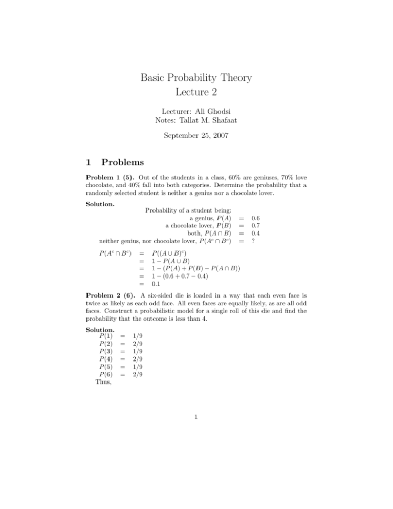
Probability of a student being:
a genius, P (A)
a chocolate lover, P (B)
both, P (A ∩ B)
neither genius, nor chocolate lover, P (Ac ∩ B c )
P (Ac ∩ B c )
=
=
=
=
=
=
=
=
=
0.6
0.7
0.4
?
P ((A ∪ B)c )
1 − P (A ∪ B)
1 − (P (A) + P (B) − P (A ∩ B))
1 − (0.6 + 0.7 − 0.4)
0.1
Problem 2 (6). A six-sided die is loaded in a way that each even face is
twice as likely as each odd face. All even faces are equally likely, as are all odd
faces. Construct a probabilistic model for a single roll of this die and find the
probability that the outcome is less than 4.
Solution.
P (1)
P (2)
P (3)
P (4)
P (5)
P (6)
Thus,
=
=
=
=
=
=
1/9
2/9
1/9
2/9
1/9
2/9
1
P ({i|i < 4})
=
=
=
=
P
P ({i})
P ({1}) + P ({2}) + P ({3})
1/9 + 2/9 + 1/9
4/9
{i|i<4}
Problem 3 (7). A four-sided die is rolled repeatedly, until the first time (if
ever) that an even number is obtained. What is the sample space for this
experiment?
Solution.
The outcome of the experiment can be an finite or an infinite sequence.
The finite sequence can be represented in the form of (i1 , i2 , . . . , in − 1, in ) such
that ik ∈ {1, 3} f or 0 ≤ k < n and in ∈ {2, 4}
The infinite sequence can be be represented in the form of (i1 , i2 , . . .)
The outcome of the experiment can also be represented as string of binary
digits: {0, 1}n, 1 ≤ n ≤ inf such that if the sequence is finite, the last digit maps
as
0⇒2
1⇒4
and for all other digits,
0⇒2
1⇒3
2
Continuous Models
Probabilistic models with continuous sample spaces differ from their discrete
counterparts in that the probabilities of the single-element events may not be
sufficient to characterize the probability law. This is illustrated in the following
example, which also indicate how to generalize the uniform probability law to
the case of a continuous sample space.
Example. Romeo and Juliet have a date at a given time, and each will
arrive at the meeting place with a delay between 0 and 1 hour, with all pairs of
delays being equally likely. The first to arrive will wait for 15 minutes and will
leave if the other has not yet arrived. What is the probability that they will
meet?
Let us use as sample space the unit square, whose elements are the possible
pairs of delays for the two of them. Our interpretation of equally likely pairs
of delays is to let the probability of a subset of be equal to its area. This
probability law satisfies the three probability axioms. The event that Romeo
and Juliet will meet is the shaded region in figure 1, and its probability is
calculated to be 7/16.
As shown in figure 1, the event M that Romeo and Juliet will arrive within
15 minutes of each other is
M = {(x, y) | |xy| ≤ 1/4, 0 ≤ x ≤ 1, 0 ≤ y ≤ 1},
2
Figure 1: State space of a continuous model for the Romeo-Juliet meeting time
example
and is shaded in the figure. The area of M is 1 minus the area of the two
unshaded triangles, or 1 (3/4)(3/4) = 7/16. Thus, the probability of meeting
is 7/16.
Bertrand’s Paradox
Probability theory is full of paradoxes in which different calculation methods seem to five different answers to the same question. Invariably though,
these apparent inconsistencies turn out to reflect poorly specified or ambiguous
probabilistic models. Here, we discuss the Bertrand’s paradox.
Presented by L. F. Bertrand in 1889, this paradox illustrates the need to
specify unambiguously a probabilistic model. Consider a circle and an equilateral triangle inscribed in the circle. What is the probability that the length of a
randomly chosen chord of the circle is greater than the side of the triangle? The
following three solutions, based on the meanings of choosing a random chord,
lead to three contradictory results.
Solution 1: Random Radius Method We take a radius of the circle, such as
AB, and we choose a point C on that radius, with all points being equally likely.
We then draw the chord through C that is orthogonal to AB. AB intersects the
triangle at the midpoint of AB, as shown below.
Area of triangle XYZ is 3-times the area of triangle XYO since △XY Z is
an equilateral triangle. Since area of △XY O is a2 and area of △XY Z is a(x+r)
,
2
thus:
3a
= a(x+r))
2
2
⇒ 2ax = ar
⇒ x = r2 ⇒ c = 2r
Since AB intersects the triangle at the midpoint, the probability that the
length of the chord is greater than the side is 1/2.
3
Solution 2: Random Endpoint Method We take a point on the circle, such
as the vertex V, we draw the tangent to the circle through V , and we draw a
line through V that forms a random angle Φ with the tangent, with all angles
being equally likely. We consider the chord obtained by the intersection of this
line with the circle. Since the triangle is equilateral, each angle of the triangle
is π3 . Thus, the length of the chord is greater that the side of the triangle if Φ is
between π3 and 2π
3 . Since Φ takes values between 0 and π, the probability that
the length of the chord is greater than the side is 31 .
Solution 3: Random Midpoint Method Choose a point anywhere within
the circle and construct a chord with the chosen point as its midpoint. The
chord is longer than a side of the inscribed triangle if the chosen point falls
within a concentric circle of radius 1/2. The area of the smaller circle is one
πr2
fourth the area of the larger circle( πr4 2 = 41 ), therefore the probability a random
chord is longer than a side of the inscribed triangle is one fourth.
Figure 2: Three solutions to the Betrand’s paradox
3
Conditional Probability
Conditional probability is a way of reasoning about the outcome of an experiment based on partial information. For instance,
1. In an experiment involving two successive rolls of a die, you are told that
the sum of the two rolls is 9. How likely is it that the first roll was a 6?
2. In a word guessing game, the first letter of the word is a ’t’. What is the
likelihood that the second letter is an ’h’ ?
3. A fair die (all six outcomes are equally likely) is rolled. If we are told that
the outcome is even, what is the probability that the outcome is 6?
4
Thus, conditional probability is the probability of an event given that another event has occurred. The conditional probability for any event A given
that event B has occured is denoted as P (A|B).
Conditional probability is defined as
P (A|B) =
P (A ∩ B)
P (B)
given that P (B) > 0. Thus, conditional probability makes sense only if something has happened, else, it is undefined.
For an experiment where all outcomes are equally likely, the conditional
probability is given as
|A ∩ B|
.
P (A|B) =
|B|
In example 3 above,
P (six|even) =
|outcome is six ∩ even|
1
=
|outcome is even|
3
Probability Axioms The conditional probability P(A—B) should form a
legitimate probability law that satifies the three axioms.
1. Non-negativity: Since neither P (A ∩ B) nor P (B) can be negative, thus
P (A∩B)
P (B) is also non-negative.
2. Additivity: This axiom states that for two disjoint events A and B (A ∩
B = ∅),
P (A ∪ B) = P (A) + P (B).
In case of conditional probability, assuming A and B are disjoint events,
we have
P (A ∪ B)
=
=
=
=
P ((A∪B)∩C)
P (C)
P ((A∩C)∪(B∩C))
P (C)
P ((A∩C)
+ P P(B∩C)
P (C)
(C)
P (A|C) + P (B|C)
Thus, the additivity axiom holds.
3. Normalization:
P (Ω|B) =
P (Ω∩B)
P (B)
=
P (B)
P (B)
=1
Since conditional probabilities constitute a legitimate probability law, all
general properties of probability laws remain valid.
5
4
Examples
Example: We toss a fair coin three successive times. We wish to find the
conditional probability P (A | B) when A and B are the events A = {more
heads than tails come up}, B = {1st toss is a head}.
Solution: The sample space consists of eight sequences, Ω = {HHH, HHT,
HTH, HTT, THH, THT, TTH, TTT}, which we assume to be equally likely.
We have, |B| = 4 and |A ∩ B| = 3
3
So, P (A|B) = |A∩B|
|B| = 4
Example: A fair 4-sided die is rolled twice and we assume that all sixteen
possible outcomes are equally likely. Let X and Y be the result of the 1st and
the 2nd roll, respectively. We wish to determine the conditional probability
P(A—B), where A = {max(X, Y ) = m}, B= {min(X, Y ) = 2}, and m takes
each of the values 1, 2, 3, 4.
Solution:
We can first determine the probabilities P (A ∩ B) and P(B) by counting the
number of elements of A ∩ B and B, respectively, and dividing by 16. Alternatively, we can directly divide the number of elements of A ∩ B with the number
of elements of B; as can be seen in figure 3.
Figure 3: State space of a 4-sided die
Sample space of an experiment involving two rolls of a 4-sided die. The
conditioning event B = min(X, Y ) = 2 consists of the 5-element shaded set.
The set A = max(X, Y ) = m shares with B two elements if m = 3 or m = 4,
one element if m = 2, and no element if m = 1. Thus, we have

if m = 3 or m = 4,
 2/5
P (max(X, Y ) = m | B) =
1/5
if m = 2,

0
if m = 1.
Example: A conservative design team, call it C, and an innovative design team,
6
call it N, are asked to separately design a new product within a month. From
past experience we know that:
(a) The probability that team C is successful is 2/3.
(b) The probability that team N is successful is 1/2.
(c) The probability that at least one team is successful is 3/4.
Assuming that exactly one successful design is produced, what is the probability
that it was designed by team N?
Solution:
Probability that the conservative team succeeds, P(C) = 32
Probability that the innovative team succeeds, P(N) = 12
Probability that atleast one is successful, P(C ∪ N) = 34
P (N |Onlyone) =?
∩OnlyOne)
P (N |Onlyone) = P (N
P (OnlyOne)
P (C ∩ N ) = P (C) + P (N ) − P (C ∪ N )
= 23 + 21 − 43
5
= 12
Only one design succeeds = (C ∩ N c ) ∪ (C c ∩ N )
= ((C ∩ N c ) ∪ C c ) ∩ ((C ∩ N c ) ∪ N )
= ((C ∪ C c ) ∩ (N c ∪ C c )) ∩ ((C ∪ N ) ∩ (N c ∪ N ))
= (Ω ∩ (N c ∪ C c )) ∩ ((C ∪ N ) ∩ Ω)
= (N c ∪ C c ) ∩ (C ∪ N )
= (N ∩ C)c ∩ (C ∪ N )
Thus, P(Only one)
and, P (N ∩ OnlyOne)
Hence, P (N |Onlyone)
=
=
=
=
=
=
P ((N ∩ C)c ∩ (C ∪ N ))
P ((N ∩ C)c ) + P ((C ∪ N )) − P ((N c ∪ C c ) ∪ (C ∪ N ))
(1 − P (N ∩ C)) + 43 − P (N c ∪ C c ∪ C ∪ N )
5
(1 − 12
) + 43 − P (Ω)
5
1 − 12 ) + 43 − 1
=
=
=
=
=
=
=
=
=
=
(C ∩ N c ) ∪ (C c ∩ N )
P (N ∩ ((N c ∪ C c ) ∩ (C ∪ N )))
P (N ∩ (C ∪ N ) ∩ (N c ∪ C c ))
P (N ∩ (N c ∪ C c ))
P ((N ∩ N c ) ∪ (N ∩ C c ))
P (∅ ∪ (N ∩ C c ))
P (N ∩ C c )
P (N ) − P (N ∩ C) because P (N ) = P (N ∩ C c ) + P (N ∩ C)
5
1
2 − 12
=
P (N ∩OnlyOne)
P (OnlyOne)
=
=
1
3
1
12
1
12
1
3
1
4
7
5
Problems
Problem 1. Prove that P (Ac |B) = 1 − P (A|B)
Problem 2. We roll two fair 6-sided dice. Each one of the 36 possible
outcomes is assumed to be equally likely. (a) Find the probability that doubles
are rolled. (b) Given that the roll results in a sum of 4 or less, find the conditional
probability that doubles are rolled. (c) Find the probability that at least one
die roll is a 6. (d) Given that the two dice land on different numbers, find the
conditional probability that at least one die roll is a 6.
Problem 3. A coin is tossed twice. Alice claims that the event of two heads
is at least as likely if we know that the first toss is a head than if we know that
at least one of the tosses is a head. Is she right? Does it make a difference if
the coin is fair or unfair? How can we generalize Alices reasoning?
8