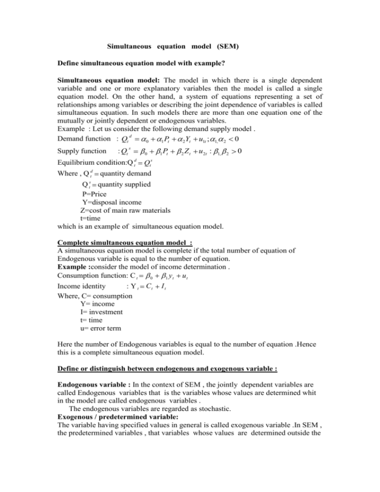
Simultaneous equation model (SEM)
Define simultaneous equation model with example?
Simultaneous equation model: The model in which there is a single dependent
variable and one or more explanatory variables then the model is called a single
equation model. On the other hand, a system of equations representing a set of
relationships among variables or describing the joint dependence of variables is called
simultaneous equation. In such models there are more than one equation one of the
mutually or jointly dependent or endogenous variables.
Example : Let us consider the following demand supply model .
d
Demand function : Qt
u1t ; 1, 2 0
0
1 Pt
2Yt
Supply function
: Qt
s
Equilibrium condition:Q td
0
P
1 t
2
Zt
u 2t :
1,
2
0
Qts
Where , Q td quantity demand
Q ts quantity supplied
P=Price
Y=disposal income
Z=cost of main raw materials
t=time
which is an example of simultaneous equation model.
Complete simultaneous equation model :
A simultaneous equation model is complete if the total number of equation of
Endogenous variable is equal to the number of equation.
Example :consider the model of income determination .
ut
Consumption function: C t
0
1 yt
Income identity
: Y t Ct
Where, C= consumption
Y= income
I= investment
t= time
u= error term
It
Here the number of Endogenous variables is equal to the number of equation .Hence
this is a complete simultaneous equation model.
Define or distinguish between endogenous and exogenous variable :
Endogenous variable : In the context of SEM , the jointly dependent variables are
called Endogenous variables that is the variables whose values are determined whit
in the model are called endogenous variables .
The endogenous variables are regarded as stochastic.
Exogenous / predetermined variable:
The variable having specified values in general is called exogenous variable .In SEM ,
the predetermined variables , that variables whose values are determined outside the
model are called exogenous variable .It is also known as non-stochastic as non
random variable .
Example: Let us consider the Keynesian model of income distribution .
ut
Consumption function : C t
0
1 yt
Income identity
: Y t Ct I t
Where ,
C =consumption expenditure
Y =Income
I =Investment
T =time
t =saving
U =stochastic disturbance term
0
1 = parameters.
In the above example, C and Y are called endogenous variables .Since they are
depending to each other and their values are determined within SEM. And I is treated
as exogenous variables its value can be determined outside the model.
Different types of Endogenous and variables .
Endogenous variables divide into two categories such as
1: Current endogenous variables.
2 : Lagged endogenous variables.
Exogenous variables also divide into two categories such as
1: Current exogenous variables.
2: Lagged exogenous variables.
What are the differences between single equation model & simultaneous equation
model?
Single equation model
Simultaneous equation model
1. The model of equation
1.The model of equation representing
representing a single relationship
among variables is called simultaneous
among variables is called single
equation model.
equation model.
2. In such model there is only one
2. In such model there is more than one
equation.
equation.
3. Example: consumption function: 3. Example: C t
ut
0
1 yt
ut
Ct
0
1 yt
Y t Ct I t
4. In this method we may use OLS
4. In this method the classical OLS
method of estimation.
method may not be applied.
5. In single equation model one can
5. In this simultaneous equation model
estimates parameters of asingle
one may not estimate the parameters for a
equation.
single equation.
Define structural model/behavior model ?
Ans . Structural model: A complete system of equation, which describes or represents
the structure of the relationship of economic variables, is called a structural model.
The endogenous variables are expressed as the function of the other endogenous
variables, predetermined variables & disturbance.
Example :
Ct
Yt
0
1
Ct
It
yt
ut
Where, C t & Y t = endogenous variable
I t = predetermined or exogenous variable
u t = stochastic disturbance form
t = time period
1 = co –efficient of endogenous variable
= co –efficient of exogenous variable
The & are known as structural parameter co efficient.
Define reduced form of a model with example.
Reduced form of a model: The reduced form model is that model in which the
endogenous variables are expressed as an explicit function of a predetermined
variable. In otherwords, a reduced form equation is one that expresses an endogenous
variable solely in terms of the predetermined variable & the stochastic disturbances.
Example : Let us consider the Keynsian model of income determination as
u t ………..(1)
Consumption function: C t
0
1 yt
Income identity
: Y t C t I t ……………….(2)
Where,
C= consumption
Y= income
I= investment
t= time
u= error term
Here , C t &Y t are the endogenous variable & I t is an exogenous variable.
Now , if we put the value of C t in equation (2),
We get,
Yt
ut I t
0
1Yt
Yt (1
Yt
Yt
Where,
1
0
1
1
0
0
0
)
,
ut
It
ut
1 1 1 1
wt .......... (3)
1It
0
It
1
1
, wt
ut
1 1
1 1
1 1
So, the equation (3) is called reduced form equation , it express the endogenous solely
as a function of the exogenous variables I & the stochastic disturbance term
wt , 0 & 1 are the reduced form parameter.
Recursive model: A model is called recursive if its structural equations can be
ordered in such a way that the first equation includes only predetermined variables in
the right hand side. The second equation contains predetermined variables & the first
endogenous variable (of the 1st equation) in the right hand side & so on. i.e
Y1 f x1 , x2 ,..., xk u1
Y2
f x1 , x2 ,..., xk ,Y1 , u 2
Y3
f x1 , x2 ,..., xk , Y1 , Y2 , u 3
And so on.
Example: As an example of recursive system, one way postulate the following model
of wage & price determination.
u1t
Price equation: P t
10
11 wt 1
12 Rt
13 M t
14 Lt
u 2t
Wage equation: W t
20
21UN t
22 Pt
Properties:
1. OLS can be applied straight a way on the each equations to estimate the
parameters.
2. OLS estimates on the parameters of recursive model is best & unbiased.
3. There is no independency among the endogenous variable in recursive model.
4. The same time period disturbances in different equations are uncorrelated. This is
the assumption of zero contemporaneous correlation.
Simultaneous equation bias:
The bias arising from the application of classical least square to an equation belonging
to a system of simultaneous relations is called simultaneous equation bias.
Because of arising:
In the one or more explanatory variables are correlated with the disturbance term
because the estimators thus obtained are inconsistent.
Consequences:
This creates several problems. Firstly these arises the problem of identification of the
parameters of individual relationships. Secondly, these arise problems of estimation.
Problem: consider the Keynsian model & show that,
1. Y t & u t are uncorrelated.
2. The OLS estimates of 1 is biased & inconsistent.
Solution : Let us consider, the Keynesian income model,
Consumption function: C t
0
1
yt
u t ………..(1)
: Y t C t I t ……………….(2)
C= consumption
Y= income
I= investment
t= time
u= error term
u t follows the following CLRM conditions.
Income identity
Where,
2
(1)E(u t )= 0, (2)E(u t2 )
(3) E( ut , ut j )
Now substituting (1) in(2) ,we get,
0 j
0 (4)COV( I t , u t )
E (u t , I t )
0
Yt
Y
0
1 t
Yt (1
1
)
It
It
ut
0
It
0
Yt
ut
1
ut
1
1
1
1
1
1
1
1
1
0
1
It
0
.......... (3)
1
It
0
E (Yt )
E (Yt )
1
.......... ...( 4)
1
Now,(3)-(4) we have,
Yt
ut
E (Yt )
Now, Cov( Yt , u t )
1
.......... .(5)
1
E[Yt
E (Yt )][u t
E (u t )]
=E[Y t -E(Y t )]u t [ E (u t )
ut
=E[
=
1
1
1
0]
]u t
1
E (u t2 )
1
2
=
0
1
1
Since 2 >0 and 0< <1
So, Y t & u t are correlated because the assumption of the CLRM are violated & hence
OLS estimators are inconsistent in this situation.
Biased of ˆ1 :
(C t Ct )(Yt Yt )
C t (Yt Yt )
(Yt Yt )C
ˆ COV (Ct , Yt ) SP(C t , Yt )
1
V (Yt )
Ct (Yt
(Yt
SS (Yt )
Yt )
Ct yt
2
y t2
Yt )
Y
0
(Yt
ut yt
1 t
y t2
ut yt
1
E ( ˆ1 )
yt
2
1
.......... .(6)
E
ut yt
y t2
1
i.e ˆ1 is not an unbiased estimator of
1
Yt ) 2
(Yt
Yt ) 2
E[ ˆ1 ]
Bias
1
ut yt
E
1
yt
1
2
ut yt
=E
yt
2
Hence, ˆ1 is a biased estimator of
1
and the amount of bias is E
ut yt
yt
2
Inconsistency of ˆ1 :
An estimator is said to be consistent if its probability limit is equal to its true value.
Taking probability limit [Plim] in the both sides of equation (6) then
Plim[ ˆ1 ]=Plim[
=
=
1
1
1
Since
2
1
+
2
2
yt / n
COV [Yt , u t ]
v(Yt )
2
=
yt
ut yt / n
+Plim
+
ut yt
]+Plim
/1
>0 and 0<
1
2
Y
<1, thus Plim[ ˆ1 ] will always be greater than
1
.
Plim[ ˆ1 ] 0
Therefore , ˆ1 is to be an inconsistent estimator.
OLS estimator is not appropriate in a simultaneous equation:
The OLS estimate method is not appropriate in a simultaneous equation model
because one or more explanatory variables are correlated with the disturbance term in
that equation & the estimator thus obtained are inconsistent. For this reason OLS
method is not appropriate in a simultaneous equation model.