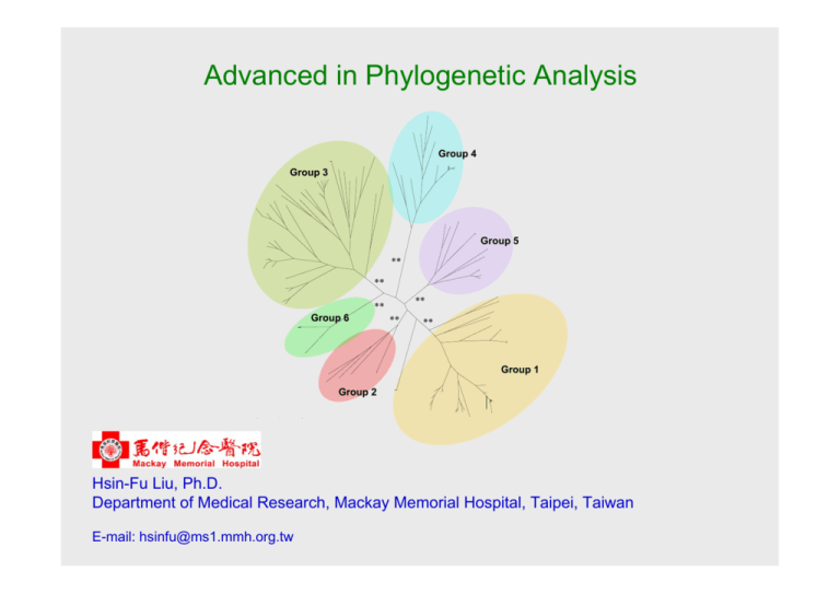
Advanced in Phylogenetic Analysis
Group 4
53A36
Group 3
Group 5
**
**
**
**
Group 6
**
53A26
**
Group 1
Group 2
53A37
.2
Hsin-Fu Liu, Ph.D.
Department of Medical Research, Mackay Memorial Hospital, Taipei, Taiwan
E-mail: hsinfu@ms1.mmh.org.tw
Application of Phylogenetic Analysis
•
•
•
•
•
•
•
•
Evolutionary studies
Classifications
Phylogeography
Phylogenomics
Molecular Epidemiology
Phylodynamics
Forensic Sciences, Criminal Investigation
etc.…….
Some of the applications need to be very precise!
Some key points for performing a phylogenetic analysis
Select an informative region to analyze
coding or non-coding region
length of the fragment
phylogenetic signal
Make an optimal sequence alignment
the bias in selecting the taxa
sequence homology
insertions or deletions
Use different methods to construct the trees
Neighbour-Joining
Maximum Parsimony
Maximum Likelihood
Bayesian
Statistical test for phylogenetic trees
bootstrapping (1000 replicates)
http://evolution.genetics.washington.edu/phylip/software.html
This site lists more than 392 phylogeny packages and 54 free servers.
Perhaps the best-known programs are PAUP* (David Swofford and
colleagues) and PHYLIP (Joe Felsenstein).
Distance matrix methods
1 TCAAGTCAGGTTCGA
2 TCCAGTTAGACTCGA
3 TTCAATCAGGCCCGA
Convert dissimilarity to evolutionary
distance by correcting for multiple events
per site according to a certain model of
evolution, e.g. Jukes and Cantor.
2
3
1
0.266
0.333
2
3
1
0.33
0.44
2
3
dissimilarity
0.333
2
0.44
3
evolutionary
distance
A first idea about the relationship among different taxa can be viewed by their evolutionary distance.
The simplest way to estimate the evolutionary distance is to count the total number of nucleotide
differences between them and divide by the total number of available sites. An evolutionary distance
obtained in such a way is called uncorrected distance or Hamming distance. A more realistic
estimation can be achieved by applying a particular model of evolution that is making assumptions on
how nucleotides change during the evolutionary process.
The simplest approach to measuring distances between sequences is to align pairs of sequences,
and then to count the number of differences. The degree of divergence is called the Hamming
distance. For an alignment of length N with n sites at which there are differences, the degree of
divergence D is:
D=n/N
But observed differences do not equal genetic distance! Genetic distance involves mutations that are
not observed directly.
Uncorrected distance vs. evolutionary distance
Jukes and Cantor (1969) proposed a corrective formula:
D = (- 3 ) ln (1 – 4 p)
3
4
Consider an alignment where 3/60 aligned residues differ. The normalized Hamming
distance is 3/60 = 0.05. The Jukes-Cantor correction is
4
D = (- 3 ) ln (1 – 0.05) = 0.052
3
4
When 30/60 aligned residues differ, the Jukes-Cantor correction is more substantial:
D = (- 3 ) ln (1 – 4 0.5) = 0.82
4
3
Ancestral
Sequence
Present
Sequences
1
A
C
T
G
A
A
C
G
T
A
A
C
G
C
A
C
T
G
G
A
G
G
A
A
T
C
G
C
2
A
A
T
G
A
A
A
G
A
A
T
C
G
C
Although only 3 nucleotide
differences can be observed,
13 mutations have occurred
during evolution.
During Evolution
Sequence 1
A
C
T
G
T
A C
A
C G
G
T A
A
T
A C
C
G
C
G
Sequence 2
A
A
C
T
G
A
A
A
C
G
A
T
A
A
T
C
G
T
C
C
Single substitution
Sequential substitutions
Coincidental substitutions
Parallel substitutions
Convergent substitutions
Back substitutions
Correcting for unobserved mutations
Expected difference
Sequence difference
Correction
Observed difference
Time/Evolutionary distance
How to correct the difference?
Apply a substitution model that tries to estimate the
correct number of substitutions.
Nucleotide substitution models
Jukes and Cantor’s

A


C

T

pyrimidines
equal substitution rate
Jukes-Cantor
(JC or JC69)
Kimura 2-Parameter
(K2P or K80)

A
purines
G


Kimura’s 2 parameter



C
G

T
unequal substitution rate
transition  transversion
one rate of substitution
equal base frequencies
two types of substitution
equal base frequencies
Felsenstein 1981
(F81)
one rate of substitution
unequal base frequencies
Hasegawa-Kishino-Yano, or Felsenstein
(HKY85 or F84)
two types of substitution
unequal base frequencies
Tamura and Nei
(TN93)
three types of substitution
unequal base frequencies
General Time Reversible
(GTR)
six types of substitution
unequal base frequencies
Among-site rate variation (Γ distribution)
α<1 is L-shaped: most of the sites are
considered to have a low substitution rate,
or they are virtually invariable, while few of
them evolve at very high rate.
α>1 is bell-shaped: most of the sites
have intermediate rates, while few of them
evolve at very low or very high rate.
All the models described in the previous section assume each site in the aligned nucleotide
sequences mutates exactly at the same rate. However, different selective pressure at different
positions of the genome can be responsible for some sites to evolve slower or faster than others. In
coding regions, mutations in first and second position generally lead to amino acid replacement and
they occur normally at slower rate due to purifying selection. On the other hand, non-coding regions
tend to change faster, because mutations can occur with less constraints than in coding ones. In a
classical approach among-site rate heterogeneity can be approximated by a statistical function called
g-distribution, which represents the nucleotide substitution rate as a function of the proportion of sites
having a particular rate. The use of g-distribution can account for two different levels of rate variation
in real data. The inclusion of g-distributed nucleotide substitution rates in the models described above
is a more realistic description of the evolutionary process and can improve the estimation of the
evolutionary distance.
Genetic Distances: Example
Genetic distance between SIVcpz and HIV-1 (p24 gene)
• observed # changes / # sites
= 0.406
• Jukes-Cantor
= 0.586
• Kimura 2 parameter
= 0.602
• Hasegawa-Kishino-Yano
= 0.611
• General reversible
= 0.620
• General reversible + gamma
= 1.017
Likelihood Ratio Test (LRT)
The performances of the different substitution models can be tested
using the likelihood ratio test
•For particular questions (e.g. molecular clock analysis) it is important to have the
correct branch length and thus it is worth to put effort in investigating the most
appropriate evolutionary model.
•Whether or not the different lineages in a phylogenetic trees are evolving at constant
rate it is possible to evaluate employing the LRT.
•Analyses of real data suggest that while different models of nucleotide substitutions
often have led to drastic changes in the likelihood of a tree or in the distance matrix of
the taxa, they have only minor effect on tree topology.
•The LRT rejects a simpler model in favor of a more complex one when the double of
the difference between the two log likelihood, calculated employing the two different
models, is significant in a 2 test. The degrees of freedom for the 2 test is given by the
difference between the number of free parameters in the more complex model and the
number of constraints in the simpler one.
Model selection
Akaike information criterion
The Akaike information criterion is a measure of the relative goodness of fit of a
statistical model. It was developed by Hirotsugu Akaike, under the name of "an
information criterion" (AIC) first published in 1974. It is grounded in the concept of
information entropy, in effect offering a relative measure of the information lost when a
given model is used to describe reality. It can be said to describe the tradeoff between
bias and variance in model construction, or loosely speaking between accuracy and
complexity of the model.
Where k is the number of parameters in the statistical model, and L is the maximized
value of the likelihood function for the estimated model.
AICc
AICc is AIC with a correction for finite sample sizes. AICc was first proposed by Hurvich
& Tsai in 1989.
When all the models in the candidate set have the same k, then AICc and AIC will give
identical (relative) valuations. In that situation, then, AIC can always be used.
Model selection
Bayesian information criterion
Bayesian information criterion (BIC) is a criterion for model selection among a finite set
of models. It is based, in part, on the likelihood function, and it is closely related to AIC.
When fitting models, it is possible to increase the likelihood by adding parameters, but
doing so may result in over-fitting. The BIC resolves this problem by introducing a
penalty term for the number of parameters in the model. The penalty term is larger in
BIC than in AIC. The BIC was developed by Gideon E. Schwarz. In fact, Akaike was so
impressed with Schwarz's Bayesian formalism that he developed his own Bayesian
formalism, now often referred to as the ABIC for "a Bayesian Information Criterion" or
more casually "Akaike's Bayesian Information Criterion".
Parameter in the model
More parameters the model uses, more powerful it does?
Bias: distance between the average estimate and truth
Variance: spread of the estimates around the truth
Statistical test for phylogenetic trees
The tree topology obtained by any of the tree-making methods should be viewed as only an estimate
of the phylogenetic relation among the taxa. Therefore, it is essential to know how much confidence
can be associated with the branch length or the appearance of a set of taxa as a monophyletic group
in a given tree.
Bootstrap analysis
Bootstrap analysis is the most often used method for statistical evaluation of phylogenies. It is used to
test the effects of sampling error on tree inference and the stability of tree nodes by calculating how
often a particular cluster in a tree appears when nucleotide sites are re-sampled with replacements
many times.
In general:
Bootstrap value > 95% : often close to 100% confidence in that branch
Bootstrap value > 75% : often close to 95% confidence in that branch
Branch can be considered as a monophyletic group.
Note:
If the original data set is biased for some reasons, a clade may be regarded as statistically significant
even if it is a wrong one. Conversely, a clade may be a correct one even if its bootstrap value is less
than 75%. This is because the original bias cannot be corrected by the re-sampling process.
Possible consequence of insufficient bootstrapping samples
Random
number
seed
Alignment not modified
Modified alignment
Bootstrapping times
Bootstrapping times
100 times 1000 times
100 times 1000 times
5
62％
69.4％
67％
70.2％
15
68％
70.1％
77％
72.7％
23
71％
67.8％
85％
74.0％
Neighbor-joining trees
Random
number
seed
Alignment not modified
Modified alignment
Bootstrapping times
Bootstrapping times
100 times 1000 times
100 times 1000 times
5
37.6％
35.1％
85％
80％
15
35.9％
37.2％
84％
80.5％
23
31.8％
33.7％
81％
80.5％
Maximum parsimony trees
Likelihood-mapping analysis
(quartet puzzling method)
Likelihood-mapping analyses can be used as a complementary approach to
solve the controversial phylogenies.
•The method is based on an analysis of the maximum likelihoods for the three fully resolved tree
topologies that can be computed for four sequences.
•The three likelihoods are represented as points inside an equilateral triangle.
•The triangle is partitioned into different regions.
•The centre of the triangle represents a star-like evolution whereas the three corners represent wellresolved phylogeny and the three intermediate regions between the corners reflect the difficulty in
distinguishing between two of the three trees.
•For more than four sequences, the different strains can be grouped into four different subsets and all
possible quartets generated by drawing one sequence from each subset can be evaluated.
•The more points distribute in a certain region of a particular corner, the bigger the support for the tree
topology joining the four subsets represented by that corner.
•If most points locate in the center of the triangle, the four subsets are independent and related by a
star-like tree.
L1
A
C
B
D
L3
L2
C
A
D
L2
B
L1
B
A
C
L3
D
Quartet puzzling method
The three corners of the triangle represent the three possible unrooted tree topologies for four taxa.
L1, L2, and L3 represent the three likelihoods of the three trees, respectively. Each length of the
perpendicular from point P to the triangle side is equal to the likelihood of the tree represented by the
opposite corner.
Quartet Puzzling Support Values
The quartet puzzling support values can be interpreted in a similar way as bootstrap values (though
they should not confused with them). Branches showing a quartet puzzling reliability > 90% can be
considered strongly supported. Branches with lower reliability (> 70%) can in principle be also
trusted but in this case it is advisable to check how well the respective internal branch does in
comparison to other branches in the tree (i.e. check relative reliability). If you are interested in a
branch with a low confidence it is also important to check the alternative groupings that are not
included in the quartet puzzling tree.
Analysis of the phylogenetic signal
The quartet puzzling approach can be used also to visualize the phylogenetic content of a
particular data set of n aligned sequences. For n sequences (n!/4!) possible quartets, exist.
When n≥11, a random sample of 10000 quartets is sufficient to obtain a comprehensive picture
of the kind of phylogenetic signal present. The more the dots in the center of the triangle, the
more the phylogenetic noise, reflecting star-like evolution, in the data set.
1
ALLELE FREQUENCY
fixed
mutation
polymorphis
m maintained
lost
mutation
0
TIME
•
•
•
•
•
Positive selective pressure: mutant is more fit
Negative selective pressure: mutant is less fit
Balancing selection: heterozygote is more fit
Most synonymous mutations can be considered neutral
Non-synonymous mutations are always subject to selective pressure
dN/dS
•Are the substitutions we observe neutral or beneficial?
•First, classify mutations as synonymous or non-synonymous
•Synonymous substitutions are likely to be neutral
•Non-synonymous substitutions may be neutral, beneficial or deleterious
•Beneficial mutations spread faster than neutral ones
•dN/dS=ratio of non-synonymous & synonymous substitution rates.
•dN/dS = 1 if all non-synonymous substitutions are neutral
•dN/dS < 1 if some non-synonymous substitutions are deleterious
•dN/dS = 0 if all non-synonymous substitutions are deleterious
•dN/dS > 1 only if some non-synonymous substitutions are beneficial
Synonymous substitutions are not always neutral
•Overlapping genes and reading frames
Very common in viruses (e.g. HTLVs)
•Secondary RNA or DNA structure
e.g. stem-loops
•Codons for the same amino acid differ in fitness
May result from different translational efficiencies of tRNAs
•Untranslated or regulatory regions
Detecting recombination in viral sequences
Consistent genome-wide HIV-1 M-group clustering
Phylogenetic analysis results in similar general clustering on HIV strains
irrespective of which region of the genome is used for the analysis.
Jumping of recombinant isolates
Recombinant isolate KAL153.
Similarity and bootscanning analysis followed by phylogenetic analysis (K2P+NJ) of the
identified segments.
Networks for analysis of recombination
Split decomposition method
Evolutionary relationships between taxa are most often represented as phylogenetic trees and this
is justified by the assumption that evolution is a branching or tree-like process. However, a set of
real data often contains a number of different and sometimes conflicting signals and thus does not
always clearly support a unique tree. The split decomposition method is a transformation-based
approach. Essentially, evolutionary data is transformed or, more precisely, "canonically
decomposed", into a sum of "weakly compatible splits" and then represented by a so-called splits
graph. For ideal data, this is a tree, whereas less ideal data will give rise to a tree-like network that
can be interpreted as possible evidence for different and conflicting phylogenies.
Neighbor-Net
Neighbor-Net, a distance based method for constructing phylogenetic networks that is based on
the Neighbor-Joining (NJ) algorithm of Saitou and Nei. Neighbor-Net provides a snapshot of the
data that can guide more detailed analysis. Unlike split decomposition, Neighbor-Net scales well
and can quickly produce detailed and informative networks for several hundred taxa.
Multilocus sequence typing (MSLT) to
classify several hundreds Salmonella
isolates. J Clin Microbiol 2002; 40: 1627-35.
Comparison of K80-based NJ tree and split-decomposition phylogenetic analysis
Split decomposition of the Human Bocavirus in Taiwan
References
Graur D and Li W-H. 2000. Fundamentals of Molecular Evolution, 2nd edition, Sinauer Associates, Sunderland, MA.
Hillis D, Moritz C, and Mable BK (eds). 1996. Molecular Systematics, 2nd edition, Sinauer Associates, Sunderland, MA.
Masatoshi Nei and Sudhir Kumar. 2000. Molecular Evolution and Phylogenetics, Oxford University Press, New York, NY.
Philippe Lemey, Marco Salemi and Anne-Mieke Vandamme (eds). 2009. The Phylogenetic Handbook : A Practical
Approach to phylogenetic analysis and hypothesis testing, Second Edition, Cambridge University Press.
Pevsner J. 2009. Bioinformatics and Functional Genomics, 2nd edition, Wiley-Blackwell.
International Bioinformatics Workshop on Virus Evolution and Molecular Epidemiology, 1995-2009, Rega Institute for
Medical Research, Katholieke Universiteit Leuven, Leuven, Belgium.
Workshop on Molecular Evolution, 1998-2008, Marine Biological Laboratory, Woods Hole, Massachusetts, USA.
Liu Hsin-Fu. 1996. Genomic diversity and molecular phylogeny of human and simian T-cell lymphotropic viruses. Thesis
submitted for the degree of “Doctor in Medical Sciences”, Faulty of Medicine, Katholieke Universiteit Leuven, Leuven,
Belgium.
Salemi Macro. 1999. Molecular investigation of the origin and genetic stability of the human T-cell lymphotropic viruses.
Thesis submitted for the degree of “Doctor in Sciences”, Faulty of Science, Katholieke Universiteit Leuven, Leuven,
Belgium.
Note: This teaching material was prepared for the workshop only, not for formal publication, therefore did not
specifically address to the references. They were all taken from the list above.