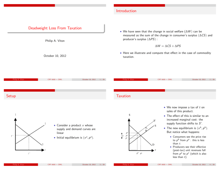
Introduction
Deadweight Loss From Taxation
We have seen that the change in social welfare (∆W ) can be
measured as the sum of the change in consumer’s surplus (∆CS ) and
producer’s surplus (∆PS ) :
Philip A. Viton
∆W = ∆CS + ∆PS
Here we illustrate and compute that e¤ect in the case of commodity
taxation.
October 10, 2012
Philip A. Viton
CRP 6600
() — DWL
October 10, 2012
1 / 29
Setup
Philip A. Viton
CRP 6600
() — DWL
October 10, 2012
2 / 29
Taxation
We now impose a tax of t on
sales of this product.
$
$
S'
S
pa
Consider a product x whose
supply and demand curves are
linear
S
t
t
Initial equilibrium is (x a , p a ).
pb
pa
pc
D
The new equilibrium is (x b , p b ).
But notice what happens:
Consumers see the price rise
to p b from p a : this is less
than t.
Producers see their e¤ective
(post-tax) unit revenues fall
from p a to p c (which is also
less than t).
D
x
x
xa
Philip A. Viton
The e¤ect of this is similar to an
increased marginal cost: the
supply function shifts to S 0 .
xb xa
CRP 6600
() — DWL
October 10, 2012
3 / 29
Philip A. Viton
CRP 6600
() — DWL
October 10, 2012
4 / 29
Tax Incidence
Consumer’s Surplus
$
This is an example of a general phenomenon: most of the time,
consumers do not bear the full burden of a commodity tax.
Some of it is absorbed by producers.
S
The proportion absorbed by producers and hence the portion passed
on to consumers depends on the relative elasticities of the demand
and supply functions.
pb
pa
pc
As always, the change in
consumer’s surplus is the area
under the demand curve
between the two price
horizontals.
In this case it is the lightly
shaded area.
D
We now return to the main thread of our analysis.
x
Note that consumers see a price
rise, hence ∆CS < 0.
xb xa
Philip A. Viton
CRP 6600
() — DWL
October 10, 2012
5 / 29
Producer’s Surplus
Philip A. Viton
October 10, 2012
6 / 29
Total Impact
$
S
pb
pa
pc
$
Producer’s surplus is the area to
the left of the supply function
between the change in producer
prices.
S
pb
pa
pc
In this case this is the darker
shaded area.
Note that producers see a price
fall, hence ∆PS < 0.
D
x
The total impact is ∆CS + ∆PS
This is shown as the shaded
areas in the …gure.
Note that both these areas a
welfare losses, and hence the
entire area has a negative sign.
D
x
xb xa
Philip A. Viton
CRP 6600
() — DWL
xb xa
CRP 6600
() — DWL
October 10, 2012
7 / 29
Philip A. Viton
CRP 6600
() — DWL
October 10, 2012
8 / 29
Impact of the Tax I
Impact of the Tax II
But what about the tax itself? Presumably we’re not just burning the
money the government takes in.
$
This is a bit subtle: we need to make an assumption about just what
the government does with the tax receipts.
For example, it would make a di¤erence (as we’ve seen) whether the
government uses its tax receipts to subsidize (reduce prices on) some
goods or services; of whether it simply returns income to the people.
S
Then tax receipts are t x b ,
the hatched rectangle in the
…gure. This is a bene…t to the
recipients, hence a positive
quantity.
pb
t pca
p
The simplest assumption is that receipts are just returned to the
people, for example, as an income tax rebate.
Assume that tax receipts are
returned to people as income.
D
x
xb xa
Philip A. Viton
CRP 6600
() — DWL
October 10, 2012
9 / 29
Deadweight Loss
Philip A. Viton
CRP 6600
() — DWL
October 10, 2012
10 / 29
Numerical Analysis
We now repeat our analysis with real numbers and functions. We assume:
$
The net impact (∆W minus tax
revenue bene…ts) is shaded.
S
pb
pa
pc
D
x
Demand:
x (p ) = 17
Note that this a negative
quantity: even after considering
the positive impact of the tax,
there is still a net welfare loss to
the community.
0.35p
Total Cost:
TC (x ) = 8 + 4x + 1.25x 2
Marginal Cost (=supply) is obtained by …nding the derivative of TC:
MC (x ) = 4 + 2.50x
This is known as the
Deadweight Loss from taxation.
Tax: we assume a tax of t = 1.25 per unit.
xb xa
Philip A. Viton
CRP 6600
() — DWL
October 10, 2012
11 / 29
Philip A. Viton
CRP 6600
() — DWL
October 10, 2012
12 / 29
Initial Equilibrium
Final Equilibrium I
Equate supply and demand, and solve for price and quantity. In this
case we insert the demand function into the supply function:
p = 4 + 2.50(17
= 46. 5
1.875p = 46.5
p = pa =
The …nal equalibrium price and quantity will be where the demand
curve interects the upward-shifted supply curve (S 0 in slide 5).
0.35p )
How do we …nd S 0 ? The marginal cost function takes an output x
and delivers a price: we have p = MC (x ).
0.875 p
46.5
= 24.80
1.875
In this case we want it to deliver a price that is t units higher, where
t is the tax.
So we focus on
To …nd the equilibrium quantity, plug the price into the demand
function:
x a = x (24.8) = 17
(0.35
p = MC (x ) + t
24.8)
= 8.32
Philip A. Viton
CRP 6600
() — DWL
October 10, 2012
13 / 29
Final Equilibrium II
Philip A. Viton
CRP 6600
() — DWL
October 10, 2012
14 / 29
Final Equilibrium III
Then S 0 is:
p = MC (x ) + t
Now plug the price into the demand function to …nd
= 4 + 2.50x + 1.25
= 5.25 + 2.50x
xb
Next, …nd the equilibrium price: equate S 0 to demand. This is parallel
to what we did before:
p = 5.25 + 2.50x
= 5.25 + 2.50(17
= 47.75 0.875p
0.35p )
pc
1.875p = 47.75
47.75
pb =
= 25. 4667
1.875
CRP 6600
() — DWL
October 10, 2012
15 / 29
25.4667)
Finally, the net price actually received by producers is the market
price less the tax, so
and solve for p (ie p b )
Philip A. Viton
= 17 (0.35
= 8. 086 67
Philip A. Viton
= pb t
= 25.4667 1.25
= 24. 216 7
CRP 6600
() — DWL
October 10, 2012
16 / 29
Equilibria Summary
Change in Consumer’s Surplus
The e¤ect of the tax on consumers is that they see prices change
from p a = 24.80 to p b = 25.4667; their consumption of x falls from
x a = 8.32 to x b = 8.08667
We have now found:
So by geometry we have
Post project equilibrium: p a = 24.80 x a = 8.32
Area of rectangle = (25.4657
Post-project equilibrium: p b = 25.4667 x b = 8.08667
Area of triangle =
1
(25.4667 24.80)
2
Post-project net price received by producers:
p b t = 25.4667 1.25 = 24. 216 7
CRP 6600
() — DWL
(8.32
8.08667 = 5. 383 296 2
8.08667) = 0.07 778 055 6
So
∆CS
Philip A. Viton
24.80)
October 10, 2012
17 / 29
Producer’s Surplus Three Ways
=
=
(5. 383 296 2 + 0.07 778 055 6)
5. 471 08
Philip A. Viton
CRP 6600
() — DWL
October 10, 2012
18 / 29
Change in Producer’s Surplus via Geometry
Producers see their price fall from x a = 24.80 to x c = 24.2167.
So by geometry we have:
We have three ways to compute the change in producer’s surplus:
Area of rectangle = (24.80
1. By geometry, since both demand and supply are linear in own-price.
2. As an integral.
Area of triangle: =
0.06 805 069 5
1
2
24.2167)
(24.80
8.08667 = 4. 716 954 6
24.2167)
(8.32
8.08667) =
So:
3. Using the fact that ∆PS = ∆Π.
∆PS
We now use our numerical example to illustrate each of these approaches.
=
=
(4. 716 954 6 + 0.06 805 069 5)
4. 785 01
This is obviously simple, but remember that it is only available in the
linear case.
Philip A. Viton
CRP 6600
() — DWL
October 10, 2012
19 / 29
Philip A. Viton
CRP 6600
() — DWL
October 10, 2012
20 / 29
Change in Producer’s Surplus as an Integral I
Change in Producer’s Surplus as an Integral II
The solution is to invert the marginal cost curve, and make it a
function of price. Solve for x:
The change in producer’s surplus is the area to the left of the supply
(=MC) function between the two price horizontals.
p = 4 + 2.50x
p
So we are looking for something like:
∆PS =
Z pc
pa
MC (p ) dp
4 = 2.50x
p 4
x =
2.50
or
The problem we now face is that our expression for marginal cost
delivers MC (a cost, or a price) as a function of output, not price:
x (p ) =
= 0.4p
MC (x ) = 4 + 2.50x
4
2.50
1
p
2.50
1.6
Then we have
MC (p ) = 0.4p
Philip A. Viton
CRP 6600
() — DWL
October 10, 2012
21 / 29
Change in Producer’s Surplus as an Integral III
S (24.80) = (0.2
Z 24.2167
(0.4p
1.6)dp
24.80
Pre-project total revenues = TR a = 8.32
1.6p and we compute the
24.802 )
(1.6 24.2167) = 78. 542 992.
(1.6 24.80) = 83. 328
= 78. 542 992
=
4. 785 01
24.80 = 206. 336.
Pre-project total costs:
TC a = TC (8.32)
= 8 + (4 8.32) + (1.25
= 127. 808
And thus:
83. 328
8.322 )
So
Πa = 206. 336
as before.
Philip A. Viton
22 / 29
Pre-project: quantity supplied = x a = 8.32. Pre-project price =
p a = 24.80. Then:
24.21672 )
∆PS
October 10, 2012
Finally, we can use the fact the ∆PS = ∆Π, and calculate pro…ts directly.
The anti-derivative is S (p ) = 0.2p 2
limits as
S (24.2167) = (0.2
CRP 6600
() — DWL
Change in Producer’s Surplus via Pro…ts I
We now want to evaluate:
∆PS =
Philip A. Viton
1.6
127. 808
= 78. 528
CRP 6600
() — DWL
October 10, 2012
23 / 29
Philip A. Viton
CRP 6600
() — DWL
October 10, 2012
24 / 29
Change in Producer’s Surplus via Pro…ts II
Change in Producer’s Surplus via Pro…ts III
Post-project quantity supplied = x b = 8.08667 ; post project (net)
producer’s price = p c = 24.2167.
Post-project total revenue:
832 46
TR b
= 8.08667
24.2167 =
RbT
Then, …nally
= 195.
∆PS
Post-project total costs:
TC b
= TC (8.086)
= 8 + (4 8.08667) + (1.25
= 122. 08947
8.086672 )
which once again agrees with our previous computations
General remark on all these calculations: there is room for di¤erences
in about the third decimal place if you round intermediate quantities
too soon.
So
Πb
Philip A. Viton
= 195. 832 46
= 73. 74299
122. 08947
CRP 6600
() — DWL
October 10, 2012
25 / 29
Welfare of Consumers and Producers
Philip A. Viton
CRP 6600
() — DWL
October 10, 2012
26 / 29
Tax Receipts
At the post-project equilibrium, people purchase (and suppliers
produce) 8.08667 units of x.
Putting all this together we have:
∆W
= ∆Π
= Πb Πa
= 73. 74299 78. 528
=
4. 78501
The unit tax is t = 1.25
= ∆CS + ∆PS
=
(5. 471 08 + 4. 78501)
=
10. 25609
So total tax receipts are
∆T
= 8.08667 1.25
= 10. 108 34
Under our assumptions, this is a direct community bene…t.
Philip A. Viton
CRP 6600
() — DWL
October 10, 2012
27 / 29
Philip A. Viton
CRP 6600
() — DWL
October 10, 2012
28 / 29
Deadweight Loss
Impact in the x-market on consumers and producers is
∆W =
10. 25609
O¤-setting tax impact:
∆T = 10. 108 34
Net impact
∆W + ∆T
=
10. 25609 + 10. 108 34
0.14775
The important thing to observe is that this is still a negative quantity,
the deadweight loss.
Philip A. Viton
CRP 6600
() — DWL
October 10, 2012
29 / 29