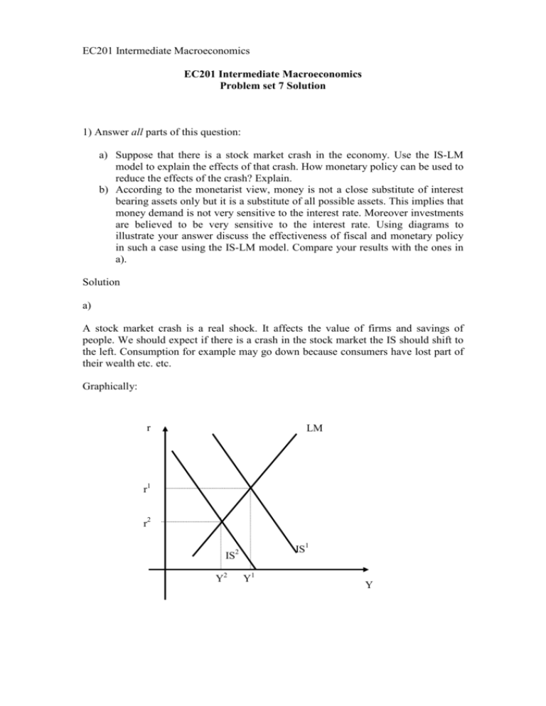
EC201 Intermediate Macroeconomics
EC201 Intermediate Macroeconomics
Problem set 7 Solution
1) Answer all parts of this question:
a) Suppose that there is a stock market crash in the economy. Use the IS-LM
model to explain the effects of that crash. How monetary policy can be used to
reduce the effects of the crash? Explain.
b) According to the monetarist view, money is not a close substitute of interest
bearing assets only but it is a substitute of all possible assets. This implies that
money demand is not very sensitive to the interest rate. Moreover investments
are believed to be very sensitive to the interest rate. Using diagrams to
illustrate your answer discuss the effectiveness of fiscal and monetary policy
in such a case using the IS-LM model. Compare your results with the ones in
a).
Solution
a)
A stock market crash is a real shock. It affects the value of firms and savings of
people. We should expect if there is a crash in the stock market the IS should shift to
the left. Consumption for example may go down because consumers have lost part of
their wealth etc. etc.
Graphically:
r
LM
r1
r2
IS1
IS2
Y2
Y1
Y
The crash in the stock market shifts the IS curve from IS1 to IS2. This results in a
decrease in equilibrium output from Y1 to Y2, and also in the equilibrium interest rate.
We have a recession in the economy.
What the central bank can do is to increase money supply so that interest rate will
decrease further trying to boost investment expenditure and so output.
Graphically:
r
LM
LM1
r1
r2
r3
IS1
IS2
Y2
Y1
Y
Money supply increases to the LM shifts to the right to LM1. There is an excess of
money supply in the money market and so the interest rate will fall. In the goods
market Investment expenditure will increase so that output will increase. In principle
we can go back to the original equilibrium of output while the equilibrium interest
rate is now much lower (r3) (if that is consistent with a positive interest rate).
Therefore in principle monetary policy can be used to offset completely the negative
effects of the shock on output.
Notice the difference with the case illustrated in Lecture 9. In that lecture the idea
was: suppose that the economy can be hit by a real shock. We don’t know in advance
if the shock is good or bad. However if the economy may face a real shock (good or
bad) the best thing to do is to keep constant money supply and let the interest rate
fluctuating. This policy, once a shock hits the economy, will minimise the output
variability.
Here we know exactly what shock is hitting the economy (in this case a crash in the
stock market) and so we can move money supply and the interest rate to offset the
effects of the shock.
b)
According to monetarists money is not just a substitute for financial assets but it is a
substitute for any possible assets (real, like a house, a car etc. etc. and financial). This
implies that money demand would not be very sensitive to changes in the interest rate
since money demand should respond to changes of all relative prices not only to the
interest rate. Money here is not only demanded for transactions as assumed by the
theory of liquidity preference. Money demand is broader here.
Therefore, the LM curve will be quite steep.
Moreover, monetarists assume that investments are sensitive to the interest rate.
In this case we have the following results:
i) Monetary policy is really effective;
ii) Fiscal policy is not effective and the crowding out is almost complete;
Fiscal policy:
LM
r
IS2
2
r
r1
IS1
2
Y1 Y
Y
An increase in government expenditure (or a decrease in taxes) results mainly in a
high equilibrium interest rate while the increase in output is very limited. Crowding
out is particularly strong.
Why? An increase in G increases Y in the goods market. The increase in Y increases
money demand in the money market. Now there is an excess of money demand in the
money market. The interest rate must increase to restore the equilibrium. Since money
demand is not very sensitive to the interest rate, the increase in the r needed to restore
the equilibrium is particularly large, so the interest rate increases substantially.
Since investments are particularly sensitive to the interest rate, the big increase in the
interest rate depresses substantially private investment and so crowding out is quite
strong here.
Monetary policy: an increase in money supply will create an excess of money supply
in the money market. The interest rate must decrease. However, since investments are
very sensitive to the interest rate, a small decrease in the interest rate will increase
investment substantially in the goods market. This is turn will increase output. The
increase in output will increase money demand and this will reduce the excess of
money supply restoring the equilibrium in the money market.
Here monetary policy is very powerful, since it affects substantially the level of
output.
LM2
LM1
r
r2
IS
r1
Y1
Y2
Y
According to Keynes instead the opposite should be true. Fiscal policy should be very
effective while monetary policy has limited power. This is an empirical issue.
In 1970 a research by Andersen and Carlson1 tried to answer the question.
They estimated using US data the following regression:
4
4
i =0
i =0
∆Yt = c + ∑ m i ∆M t −i + ∑ ei ∆G t −i
In practice they wanted to see how changes in money supply ∆M t −i in and in
government expenditure ∆Gt −i can create changes in current output ∆Yt . Notice that
also changes in previous periods (t-i) are considered (this is to test if changes in, for
example, last year money supply has an effect on this year output etc. etc.)
The equation above is now known as the “St. Louis Model”. They found that all the
m i where different from zero and significant, while the ei where insignificant and so
close to zero. Thus according to this result monetary policy was very powerful since it
had a significant impact on output while government expenditure did not have any
significant impact on output.
This result would then imply that the monetarist view should be the correct one.
However, if you try to estimate the same equation using a different sample you may
find different results. Indeed this has been done. This is to say that the empirical
evidence is still inconclusive.
1
Anderson L.C. and K.M. Carlson (1970) “A Monetarist Model for Economic Stabilization”, Federal
Reserve Bank of St. Louis Review, n. 52, pp. 7-25.
2) (Taylor Rule in the IS-LM model) Consider an economy where the central bank
pursue a Taylor Rule and not a monetary targeting strategy (meaning we replace the
LM curve with the TR curve). The Taylor Rule is given by: i = i + β (Y − Y )
Where i is the nominal interest rate, i is the natural interest rate, (Y − Y ) is the
deviation of real output from the natural level and β is a positive constant that
measures the sensitivity of the interest rate setting to output deviations.
a) Assume that output is at the natural level; show graphically what the
implication for the TR curve of an increase in the sensitivity to output
deviations is.
b) Consider an increase in government expenditure in the IS-TR model. Using
diagrams to illustrate your answer show what happens to output and the
interest rate when the TR schedule is horizontal. What are the main
differences with the case where the TR schedule is upward sloping?
Solution
a)
When the central bank’s sensitivity to the output gap rises, the TR schedule becomes
steeper. Why? As β increases, central bank cares more about output deviations.
For example, suppose that Y becomes lower than the natural level; then the central
bank decreases the interest rate (according to the Taylor Rule) by a large amount in
order to bring back Y to the natural level. This means that the TR curve is quite steep.
Graphically, starting with a given TR curve, an increase in β will mean that the TR
curve rotates anti-clockwise, but around which point?
We know that if Y is at the natural level, then the central bank will set the interest rate
at its neutral level i . This corresponds to point A in the figure below. It follows that a
change of responsiveness to the output gap is represented by a rotation of TR around
point A.
b)
When the TR is horizontal it means that β = 0 , the central bank does not care about
output gap and so the interest rate is always at the natural level: i = i . If G increases,
IS shifts to the right, output increases but the interest remains constant. How the
central bank keeps the interest rate constant? The increase in G increases Y in the
goods market. The increase in Y increases money demand in the money market. Now
there is an excess of money demand in the money market. Without any intervention
by the central bank the interest rate will increase to restore equilibrium. For the
interest rate to remain constant the central bank must accommodate that increase in
money demand by increasing money supply. Now money supply is endogenous and it
changes in order to restore the equilibrium in the money market.
When TR is positively sloped, an increase in G increases output but also the interest
rate like in the usual IS-LM model. However the mechanism is now different.
Suppose we start at point A where output is at the natural level. The increase in G
increases Y in the goods market and so now the output gap increases. The increase in
Y increases money demand in the money market. Now there is an excess of money
demand. Without any intervention of the central bank the interest rate will increase to
restore equilibrium. Since the central bank cares about output gap now, it will
increase the interest rate according to the Taylor Rule in order to reduce the output
deviation and so it will move money supply in such a way that the interest rate will be
the one implied by the Taylor Rule. Money supply is again endogenous. Notice that
here we have crowding out (interest rate goes up and investment goes down), but now
it is the central bank that creates the crowding out effect by increasing the interest rate
according to the Taylor Rule.
3) Consider the following modified version of the IS-LM model:
C = 150 + 0.5(Y − T )
T = G = 300
I = 150 + 0.3Y − 10000 ρ
ρ =i+x
D
M 
  = 2Y − 20000 i
 P 
M
= 2600
P
a) Assume that the spread x is zero. Derive the IS relation and find the
equilibrium level of output (Y) and the interest rate (i) implied by the IS-LM
model.
b) Now assume that there is a fall in the firm’s capital with the result that x is
increased to 0.5%. What happens to the cost of bank loans? Calculate the new
equilibrium in the IS-LM model. Briefly explain your findings.
Solution
a) When x = 0 the IS equation is:
Y = 150 + 0.5Y − 150 + 300 + 150 + 0.3Y − 10000 i
Solving that for i:
10000 i = 450 − 0.2Y
i = 0.045 − 0.00002 Y
The LM curve is: 2600 = 2Y − 20000 i . Solving that for i:
i = −0.13 + 0.0001Y
The equilibrium is found by solving the two equations (IS and LM) simultaneously:
Y * = 1458 .3
i * = 0.016
b)
Now x =0.5%, or x =0.005. The cost of bank loans increases.
The IS becomes:
Y = 150 + 0.5Y − 150 + 300 + 150 + 0.3Y − 10000 i − 50
Solving that for i:
i = 0.04 − 0.00002 Y
The LM is the same as before: i = −0.13 + 0.0001Y
The equilibrium is now:
Y * = 1416 .7
i * = 0.012
Output decreases since investment decreases (the cost of bank loan has increased
since x has increased). The equilibrium interest rate also decreases. Graphically, this
is equivalent to a shifts to the left of the IS curve along a given LM curve.
In equilibrium the value of ρ is: ρ * = i * + x = 0.012 + 0.005 = 0.017 . The cost of bank
loan increases in equilibrium (from 0.016 to 0.017).