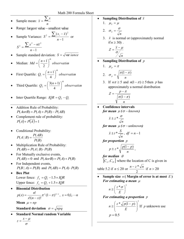



Sample mean: x 

n
Range: largest value  smallest value
Sample Variance: S 2 
S2 

x
Math 200 Formula Sheet
x
2
 nx
 (x
i
 x)
2.  x 
2
n 1
Sampling Distribution of x
1.  x  
n
3. x is normal or (approximately normal
if n  30) .
x
Z
or
2
n 1
Sample standard deviation: S  var iance

 n 1
Median: Md  
 observation
 2 

 n 1
First Quartile: Q1  
 observation
 4 

 3(n  1) 
Third Quartile: Q3  
 observation
 4 

Inter Quartile Range: IQR  Q3  Q1

Addition Rule of Probability:
P( AorB)  P( A)  P(B)  P( AB)
Complement rule of probability:
P  A  P  A   1
th



n
Sampling Distribution of p
1.  p  
th
2.  p 
th







Conditional Probability:
P( AB)
P( A | B) 
P( B)
Multiplication Rule of Probability:
P( AB)  P( A | B)  P(B)
For Mutually exclusive events,
P( AB)  0 and P( AorB)  P( A)  P(B)
For Independent events,
P(B | A)  P( B) and P( AB)  P( A)  P( B)
Box Plot
Lower fence: f L  Q1  1.5  IQR
Upper fence: f u  Q3  1.5  IQR
Binomial Distribution
n!
p ( x) 
 x (1   ) n x , x  0,1,n
x!(n  x)!
Mean   np
Standard deviation   npq

Standard Normal random Variable
x
z


 (1   )
n
3. If n  5 and n(1   )  5 then p has
approximately a normal distribution
p 
Z
 (1   )
n
Confidence intervals
for mean  (   known )
x  z*

n
for mean  (   unknown)
S
, df  n  1
x t*
n
for proportion p
p z*
p (1  p )
,
n
for median 
C L , C H  where the location of C is given in
n z* n
if n  20
2
Sample size n ( Margin of error is at most E )
For estimating a mean 
table 5.2 if n  20 or

 z * 
n

 E 
For estimating a proportion p
2
2
 z * p (1  p ) 
 If p unknown use
n


E


p  0.5
Math 200 Formula Sheet
Test Statistics for Hypothesis Testing:
For a mean 
x  0
t
df  n  1
S
n
For a proportion p
Z
 S 12 S 22 


n n 
2 
 1
df 
 0 (1   0 )
n
Inferences about  1   2 (equal Variance)
Confidence Interval
1
1
where
x1  x2  t * S p

n1 n2
Pooled variance is given by
(n1  1) S12  (n 2  1) S 22
2
and df  n1  n 2  2 .
Sp 
n1  n 2  2
Test Statistics for pooled t-test
x  x2   d 0
t 1
df  n1  n 2  2
1
1
Sp

n1 n2
Paired data
Confidence Interval
S
D  t / 2 D df  n 1
n
Hypothesis Testing
Test Statistics
D  d0
t
df  n 1
SD
n
2
2
2
rounded down to the
Test Statistics
x  x2   d 0
t 1
degrees of freedom as above.
S12 S 22

n1 n2
Bivariate Data
SS ( x)   x  nx    x
2
i
2
2
 x 

2
2
i
SS ( y )   y  n y    y
2
i
i
n
 y 

2
2
i
SS ( xy)   xi yi  nx  y    xi2 
Correlation Coefficient
r
Inference about p1  p 2
Confidence Interval
1
n2
2
2
S

S

 n 
 n 
1
2



n1  1
n2 1
nearest integer.
2
1
( p1  p 2 )  z *
S12 S 22

where
n1 n 2
x1  x 2  t *
p 0
Test Statistics
p1  p 2
Z
p (1  p ) n11 
Inferences about  1   2 (unequal Variance)
Confidence Interval
SS ( xy)
SS ( x)  SS ( y)
Regression:
p1 (1  p1 ) p 2 (1  p 2 )

n1
n2
, where p 
x1  x 2
n1  n 2
yˆ  b0  b1 x where
SS ( xy)
slope b1 
,
SS ( x) SS ( y)
intercept b0  y  b1 x
i
n
 x  y 
i
i
n