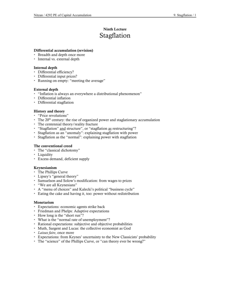
Nitzan / 4292 PE of Capital Accumulation
9. Stagflation / 1
Ninth Lecture
Stagflation
Differential accumulation (revision)
 Breadth and depth once more
 Internal vs. external depth
Internal depth
 Differential efficiency?
 Differential input prices?
 Running on empty: “meeting the average”
External depth
 “Inflation is always an everywhere a distributional phenomenon”
 Differential inflation
 Differential stagflation
History and theory
 “Price revolutions”
 The 20th century: the rise of organized power and staglationary accumulation
 The centennial theory/reality fracture
 “Stagflation” and structure”, or “stagflation as restructuring”?
 Stagflation as an “anomaly”: explaining stagflation with power
 Stagflation as the “normal”: explaining power with stagflation
The conventional creed
 The “classical dichotomy”
 Liquidity
 Excess demand, deficient supply
Keynesianism
 The Phillips Curve
 Lipsey’s “general theory”
 Samuelson and Solow’s modification: from wages to prices
 “We are all Keynesians”
 A “menu of choices” and Kalecki’s political “business cycle”
 Eating the cake and having it, too: power without redistribution
Monetarism
 Expectations: economic agents strike back
 Friedman and Phelps: Adaptive expectations
 How long is the “short run”?
 What is the “normal rate of unemployment”?
 Rational expectations: subjective and objective probabilities
 Muth, Sargent and Lucas: the collective economist as God
 Laissez faire, once more
 Expectations: from Keynes’ uncertainty to the New Classicists’ probability
 The “science” of the Phillips Curve, or “can theory ever be wrong?”
Nitzan / 4292 PE of Capital Accumulation
Supply shocks
 Stagflation: an upward slopping Phillips Curve?
 The postmodern “other”: blame it on the oil sheiks, the weather and the workers
 Oil sheiks and the whether: do raw material prices cause inflation?
 Do workers cause inflation?
 “Wage push” or “profit push”?
 “Markup inflation” and “barriers to entry”
Inflation and redistribution
 Barking up the wrong tree
 Inflation as restructuring
 Where is politics?
 Redistribution: capitalists contra workers
 Redistribution: large vs. small firms
 Why stagflation – “return” and “risk”
Regimes of differential accumulation
 The pendulum of breadth and depth
9. Stagflation / 2
Nitzan / 4292 PE of Capital Accumulation
9. Stagflation / 3
Differential Earnings
earningsD  employoment D  earnings per employeesD
Table 1
Regimes of Differential Accumulation
External
Internal
Breadth
Green-field
Mergers &
Acquisitions
Depth
Stagflation
Cost-cutting
1,000.0
log scale
1999
218%
100.0
trend growth rate:
3.4% per annum
10.0
1.0
Buy-to-Build Indicator
(mergers & acquisitions as a per cent
of gross fixed private domestic investment)
1896
0.3%
www.bnarchives.net
0.1
1880
FIGURE 1
1900
1920
1940
1960
1980
2000
2020
U.S. Accumulation: Internal vs. External Breadth
NOTE: Indicator is based on splicing of separate series.
SOURCE: Jonathan Nitzan and Shimshon Bichler, Capital as Power. A Study of Order and Creorder
(New York and London, Routledge, 2009), Ch. 15, Data Appendix.
Nitzan / 4292 PE of Capital Accumulation
9. Stagflation / 4
“Running on empty”
“How do you build a company, when your buyers are infinitely knowledgeable and where your
suppliers maintain a level playing field for your competitors? What remains your competitive
differentiator or your source of value or whatever academic cliché you want to wrap around it?”
Andrew Grove, Chairman of Intel. Cited in Byrne, John A. 2000. Visionary vs.
Visionary. Business Week, August 28, pp. 210-212.
10,000
log scale
Price increase from 1900 to 2010: 6,121%
1,000
Price increase from 1300 to 1900: 769%
100
1900
10
www.bnarchives.net
1
1200
FIGURE 2
1300
1400
1500
1600
1700
1800
1900
2000
2100
Consumer Prices in the U.K.
SOURCE: Updated from Jonathan Nitzan and Shimshon Bichler, Capital as Power: A Study of Order and Creorder
(New York and London: Routledge, 2009), Figure 16.1 p. 367. Original data from Global Financial Data (series
code: CPGBRM) (Historical data from David Hackett Fischer. 1996. The Great Wave. Price Revolution
and the Rhythm of History. New York and Oxford: Oxford University Press); IMF International
Financial Statistics through Global Insight (series code: L64@C12).
Nitzan / 4292 PE of Capital Accumulation
FIGURE 3
9. Stagflation / 5
The Seeds of Differential Stagflation
SOURCE: Means, Gardiner C. 1935. Price Inflexibility and Requirements of a Stabilizing Monetary
Policy. Journal of the American Statistical Association 30 (190, June): 401-413.
Nitzan / 4292 PE of Capital Accumulation
9. Stagflation / 6
.
IMPLICIT GDP DEFLATOR (annual % change)
8
`
6
4
2010
2
0
-2
-4
www.bnarchivs.net
-6
-1
0
1
2
3
4
5
6
7
8
9
GDP IN CONSTANT PRICES (annual % change)
FIGURE 4
United States: Inflation and Growth, 1809-2010
NOTE: Series are shown as 20-year moving averages. The straight line running through the observations is
drawn free hand for illustration purposes.
SOURCE: Updated from Jonathan Nitzan and Shimshon Bichler, Capital as Power: A Study of Order and Creorder
(New York and London: Routledge, 2009), Figure 16.4 p. 377. Historical data till 1928 are from Global Financial
Data (series code: GDPUSAM for GDP). From 1929 onward, data are from the U.S. Department of Commerce
through Global Insight (series codes: GDP for GDP; PDIGDP for the implicit GDP deflator).
Nitzan / 4292 PE of Capital Accumulation
9. Stagflation / 7
1,000
log scale
Prices* (Annual % Change)
1984
100
1956
10
1967
1972
2000
1
0
2
4
6
8
10
Real GDP (Annual % Change)
FIGURE 5
Israel: Long-Term Inflation and Growth
NOTE: Series are shown as 5-year moving averages.
SOURCE: Israel Central Bureau of Statistics.
12
14
Nitzan / 4292 PE of Capital Accumulation
9. Stagflation / 8
The neutrality of money
“There cannot, in short, be intrinsically a more insignificant thing, in the economy of society, than
money.”
John Stuart Mill
“Money is a veil.”
Irving Fisher
“Money is neutral, a veil with no consequences for real economic magnitudes.”.
Franco Modigliani
“Inflation is always an everywhere a monetary phenomenon.”
Milton Friedman
Nitzan / 4292 PE of Capital Accumulation
9. Stagflation / 9
The quantity theory of money
[P = prices, T = transactions, M = money, V = velocity, Q = output; lower case variables represent
rates of change]
1. P * T ≡ M * V
2. P ≡ M * V / T
3. p ≈ m + v – t
4. p ≈ m – t
;v=0
5. p ≈ m – q
;t=q
12
12
percent
percent
10
10
8
GDP Deflator
(annual % change)
+25%
GDP Deflator
(annual % change)
8
6
6
4
4
2
2
0
0
-2
-2
-4
-6
bnarchives.net
-6
1950
1960
1970
FIGURE 6
1980
1990
Liquidity
M1 / Real GDP
(annual % change)
-4
Liquidity
Monetary Base / Real GDP
(annual % change)
2000
2010
2020
bnarchives.net
-8
1950
1960
1970
1980
United States: Liquidity and inflation
NOTE: Annual data smoothed as 5-year moving averages. Last data points are for 2010.
SOURCE: IMF.
1990
2000
2010
2020
Nitzan / 4292 PE of Capital Accumulation
FIGURE 7
9. Stagflation / 10
The Phillips Curve
SOURCE: Phillips, A. W. 1958. The Relation Between Unemployment and the Rate of Change of
Money Wages in the United Kingdom, 1861-1957. Economica New Series 25 (100, November): 283299
Nitzan / 4292 PE of Capital Accumulation
9. Stagflation / 11
From wage inflation to price inflation
W is the wage rate, U is the rate of unemployment, P is the price level, Q is output per worker
(labour productivity), K is the markup, and lower-case variables denote corresponding rates of
change.
1. w  f U 
2. P  1  K 
W
Q
  
3. p  1  K   w  q


If the markup is fixed, we have,
4. w  p  q
Substituting into equation 1:
5. p  f U   q
Wage Inflation (w ) and Price Inflation (p ) (%)
30
20
10
w = f (U )
q
0
q
p = f (U ) - q
-10
0
2
4
6
8 10 12 14 16 18 20 22 24 26 28 30 32 34 36 38 40
Unemployment (%)
Cost push and the end of perfect competition
“Some holders of this view [cost push] attribute the push to wage boosts engineered unilaterally by
strong unions. But others give as much or more weight to the co-operative action of all sellers –organized
and unorganized labor, semimonopolistic managements, oligopolistic sellers in imperfect commodity
markets – who raise prices and costs in an attempt by each to maintain or raise his share of national
income, and who among themselves, by trying to get more than 100 per cent of the available output,
create ‘seller’s inflation . . . to explain possible cost-push inflation, it would seem more economical from
the very beginning to recognize that imperfect competition is the essence of the problem and drop the
perfect competition assumptions.”
Samuelson, Paul A., and Robert M. Solow. 1960. Problem of Achieving and
Maintaining a Stable Price Level: Analytical Aspects of Anti-Inflation Policy. The
American Economic Review 50 (2. May): 177-194
Nitzan / 4292 PE of Capital Accumulation
9. Stagflation / 12
“Expectations Augmented Phillips Curve”
pt  f1 U t   pte
pte  f 2  pt 
30
Long-Run Phillips Curve
Price Inflation (%)
20
10
0
Natural rate of unemployment
-10
0
2
4
6
8
10
12
14
16
18
20
22
24
26
Unemployment (%)
28
30
32
34
36
38
40
Nitzan / 4292 PE of Capital Accumulation
9. Stagflation / 13
Rational Expectations
“. . . expectations of firms (or, more generally, the subjective probability distribution of
outcomes) tend to be distributed, for the same information set, about the prediction of the
theory (or the ‘objective’ probability distributions of outcomes).”
Muth, John F. 1961. Rational Expectations and the Theory of Price Movements.
Econometrica 29 (3, July): 315-335.
“. . . expectations of inflation are assumed to be endogenous to the system in a very particular
way: they are assumed to be ‘rational’ in Muth’s sense – which is to say that the public’s
expectations are not systematically worse that the predictions of economic models. This
amounts to supposing that the public expectations depend, in the proper way, on the things that
economic theory says they ought to.”
Sargent, Thomas J. 1973. Rational Expectations, the Real Rate of Interest, and the
Natural Rate of Unemployment. Brookings Papers on Economic Activity (2): 429-472.
pte  E  pt I t 1 
pt  E  pt I t 1   u t
pt  pte  u t
Nitzan / 4292 PE of Capital Accumulation
9. Stagflation / 14
General Government Final Consumption Expenditure
(% of GDP)
24
22
20
18
High Income
Countries
16
14
12
10
8
Low and Middle
Income Countries
6
4
2
0
1950 1955 1960 1965 1970 1975 1980 1985 1990 1995 2000 2005 2010 2015
NOTE: Cutoff point between Middle and High Income countries: $12,276 Gross National
Income per Capita in 2010 (using the World Bank Atlas Method).
(http://siteresources.worldbank.org/DATASTATISTICS/Resources/CLASS.XLS)
SOURCE: World Development Indicators 2011
Price Inflation (%)
Nitzan / 4292 PE of Capital Accumulation
9. Stagflation / 15
Original Phillips Curve?
`
Price Inflation (%)
Unemployment (%)
Adaptive Expectations?
`
Price Inflation (%)
Unemployment (%)
Rational Expectations?
`
Unemployment (%)
Nitzan / 4292 PE of Capital Accumulation
9. Stagflation / 16
Supply Shocks: The Usual Suspects
“A clear and central villain of the piece is the historically unprecedented rise in commodity
prices (mainly food and oil) in 1973-74 and again in 1979-80 that not coincidentally
accompanied the two great burst of stagflation.
“. . . one of the variables that set the stage for the 1970s stagflation was the rise in union power
and militancy at the end of the 1960s. . . . A real wage boom resulted, which started a squeeze
on profits even before 1973. . . . It strikes us as misguided to consider the labor market as a
perfectly competitive bourse when in almost every OECD economy much of the labor force is
unionized and governments play an enormous role in affecting labour compensation.”
Bruno, Michael, and Jeffrey Sachs. 1985. Economics of Worldwide Stagflation.
Cambridge, Mass.: Harvard University Press, p. 7
Supply Shocks: The Cruel Dilemmas
“The limited capability of policy to influence supply poses a particularly vexing problem in a
stagflationary world since any stabilization policy adopted in response to stagflation is bound to
aggravate one of the problems [inflation or unemployment] even as it helps cure the other. Such
is the policy dilemma of stagflation.”
Blinder, Alan S. 1979. Economic Policy and the Great Stagflation. New York: Academic
Press, pp 20-21.
Nitzan / 4292 PE of Capital Accumulation
9. Stagflation / 17
100,000
index
log scale
CPI
10,000
Crude
Pretroleum
1,000
Food
1957=100
100
bnarchives.net
10
1950
FIGURE 8
1960
1970
1980
1990
2000
2010
2020
World prices
SOURCE: Jonathan Nitzan and Shimshon Bichler, The Global Political Economy of Israel (London:
Pluto Press, 2002), Figure 4.9, p. 164. Original data are from IMF International Financial Statistics
through Global Insight (series codes: L64@C001 for the CPI; L76AA&D@C001 for crude petroleum;
L76EX&D@C001 for food). The last data points are for 2010.
Nitzan / 4292 PE of Capital Accumulation
9. Stagflation / 18
10
8
80
GDP Deflator
(annual % change, left)
75
6
4
70
2
65
0
Compesnation of Employees /
Net National Income at Factor Cost
(% right)
-2
60
-4
-6
1930
FIGURE 9
1940
1950
1960
1970
1980
1990
2000
2010
Inflation and the Wage Share in the United States
SOURCE: U.S. Bureau of Economic Analysis. Last data points are for 2010.
55
2020
Nitzan / 4292 PE of Capital Accumulation
9. Stagflation / 19
45
1,000
log scale
GDP Deflator
(annual % change, right)
40
Gross Wages / GDP
(%, left)
100
35
30
10
25
Net Wages / GDP
(%, left)
20
1960
FIGURE 10
1965
1970
1975
1980
1985
1990
1995
2000
1
2005
Inflation and the Wage Share in Israel
SOURCE: Jonathan Nitzan and Shimshon Bichler, The Global Political Economy of Israel (London:
Pluto Press, 2002), Figure 4.7, p. 157. Original data from Bank of Israel. Israel Central Bureau of
Statistics
Nitzan / 4292 PE of Capital Accumulation
9. Stagflation / 20
Wage push or profit push?
Price = Unit Wage + Unit Profit
P=W+∏
P = (1+K) * W where K = ∏/W
 “Wage push” inflation can occur only if K is fixed.
 If K is fixed, the rates of change of profit and of wages are the same.
 If the two rates of change are the same, “wage push” inflation must also be “profit push” inflation.
Nitzan / 4292 PE of Capital Accumulation
9. Stagflation / 21
5.0
35
Corporate Earnings per
Share / Wage Rate*
(Index, right)
30
4.5
4.0
25
3.5
20
1985
1995
2005
2015
15
3.0
10
2.5
5
2.0
0
1.5
Wholesale Price Index
(annual % change, left)
-5
1.0
www.bnarchives.net
-10
1940
FIGURE 11
1950
1960
1970
1980
1990
2000
2010
0.5
2020
U.S. Inflation and Capital-Labour Redistribution
* Corporate earnings per share are for the S&P 500. The wage rate is the average hourly earnings in the goods
producing private sector till 1963 and in the private sector afterwards.
NOTE: Series are expressed as 3-years moving averages. Last data points are for 2011.
SOURCE: Updated from Jonathan Nitzan and Shimshon Bichler, Capital as Power: A Study of Order and Creorder
(New York and London: Routledge, 2009), Figure 16.2 p. 371. Original data from Standard & Poor’s through
Global Insight (series code: EARN500NS for S&P 500 earnings per share); U.S. Department of Commerce and
U.S. Bureau of Labor Statistics through Global Insight (series codes: AHPGP and AHPEAP for the wage rate;
WPINS for the wholesale price index).
Nitzan / 4292 PE of Capital Accumulation
9. Stagflation / 22
4. U.S. Inflation, Profits and Wages
(annual % change, left)
(index, right)
www.bnarchives.net
SOURCE: IMF: L64@C111 (consumer prices), L65EY@C111 (hourly wage);
Compustat: I0010 (S&P 500 Composite).
FIGURE 12
U.S. Inflation and Capital-Labour Redistribution
SOURCE: Nitzan, Jonathan, and Shimshon Bichler. 2006. Cheap Wars. Tikkun, August, 9.
Nitzan / 4292 PE of Capital Accumulation
9. Stagflation / 23
25
4.0
Wholesale Price Index
(annual % change, left)
20
3.5
3.0
15
2.5
2008
10
2.0
5
2005
1.5
0
1.0
-5
0.5
Differential Markup:
Fortune 500 / Business Sector *
(right)
-10
0.0
www.bnarchives.net
-15
1950
FIGURE 13
1960
1970
1980
1990
2000
2010
-0.5
2020
U.S. Inflation and Differential Accumulation
* The markup is the per cent of net profit in sales. The Fortune 500 markup is the per cent of after tax profit in
sales revenues. The business sector markup is computed by dividing total corporate profit after tax with IVA and
CCA (from the national income accounts) by total business receipts (from the IRS). The Differential Markup is
given by dividing the Fortune 500 markup by the business sector markup.
NOTE: Until 1993, the Fortune 500 list included only industrial corporations (firms deriving at least half their
sales revenues from manufacturing or mining). From 1994 onward, the list includes all corporations. For 1992-3,
data for Fortune 500 companies are reported without SFAS 106 special charges.
SOURCE: Jonathan Nitzan and Shimshon Bichler, Capital as Power: A Study of Order and Creorder (New York and
London: Routledge, 2009), Figure 16.3 p. 373. Original data from the U.S. Department of Commerce through
Global Insight (series codes: ZAECON for total corporate profit after tax with IVA and CCA; WPINS for the
wholesale price index); U.S. Internal Revenue Service; Fortune.
Nitzan / 4292 PE of Capital Accumulation
FIGURE 14
9. Stagflation / 24
Stagflation Index
NOTE: Stagflation Index = (standardized inflation – standardized growth) / 2. Series are measured as 12-month
% change and shown as 3-year moving averages.
SOURCE: IMF (codes: L64_A_C110 for CPI; L66_N_I_A_C110 for Industrial Production).
Nitzan / 4292 PE of Capital Accumulation
9. Stagflation / 25
2
10,000.0
log scale
Stagflation Index *
(Unemployment plus Inflation, right)
1
1,000.0
0
2007
2007
100.0
-1
-2
10.0
-3
1.0
Amalgamation Index **
(Buy-to-Build Indicator, left)
-4
www.bnarchives.net
0.1
1880
FIGURE 15
1900
1920
1940
1960
1980
2000
2020
-5
2040
Amalgamation and Stagflation in the U.S.A.
* Computed as the average of: (1) the standardised deviations from the average rate of unemployment; and (2)
the standardized deviation from the average rate of inflation of the GDP implicit price deflator.
** Mergers and acquisitions expressed as a per cent of gross fixed private domestic investment.
NOTE: Series are shown as 5-year moving averages (the first four observations in each series cover data to that
point only).
SOURCE: Jonathan Nitzan and Shimshon Bichler, Capital as Power: A Study of Order and Creorder (New York and
London: Routledge, 2009), Figure 17.1 p. 384. The stagflation index is computed based on data from the U.S.
Department of Commerce through Global Insight (series codes: RUC for the rate of unemployment since 1929;
PDIGDP for the GDP implicit price deflator); Historical Statistics of the United States (series D-8, p. 126 for the rate
of unemployment before 1929). For details on the Amalgamation Index, see the Appendix to Chapter 15 in
Nitzan and Bichler, Capital as Power. A Study of Order and Creorder.