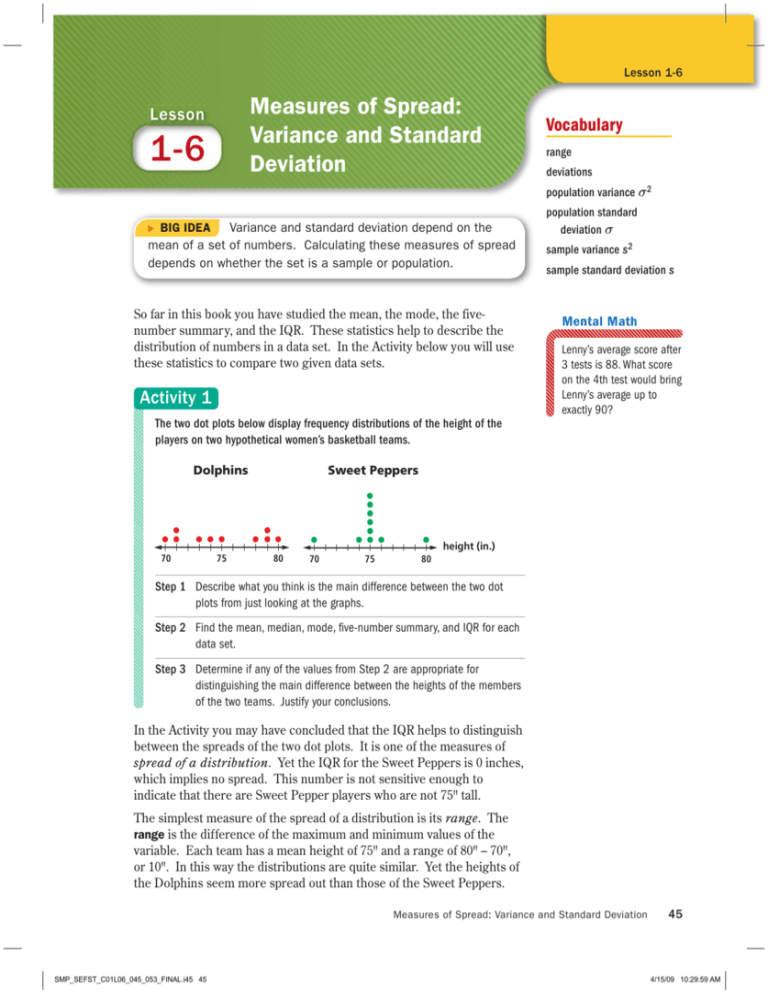
Lesson 1-6
Measures of Spread:
Variance and Standard
Deviation
Lesson
1-6
Vocabulary
range
deviations
population variance σ 2
Variance and standard deviation depend on the
mean of a set of numbers. Calculating these measures of spread
depends on whether the set is a sample or population.
BIG IDEA
So far in this book you have studied the mean, the mode, the fivenumber summary, and the IQR. These statistics help to describe the
distribution of numbers in a data set. In the Activity below you will use
these statistics to compare two given data sets.
Activity 1
population standard
deviation σ
sample variance s 2
sample standard deviation s
Mental Math
Lenny’s average score after
3 tests is 88. What score
on the 4th test would bring
Lenny’s average up to
exactly 90?
The two dot plots below display frequency distributions of the height of the
players on two hypothetical women’s basketball teams.
Dolphins
Sweet Peppers
height (in.)
70
75
80
70
75
80
Step 1 Describe what you think is the main difference between the two dot
plots from just looking at the graphs.
Step 2 Find the mean, median, mode, five-number summary, and IQR for each
data set.
Step 3 Determine if any of the values from Step 2 are appropriate for
distinguishing the main difference between the heights of the members
of the two teams. Justify your conclusions.
In the Activity you may have concluded that the IQR helps to distinguish
between the spreads of the two dot plots. It is one of the measures of
spread of a distribution. Yet the IQR for the Sweet Peppers is 0 inches,
which implies no spread. This number is not sensitive enough to
indicate that there are Sweet Pepper players who are not 75" tall.
The simplest measure of the spread of a distribution is its range. The
range is the difference of the maximum and minimum values of the
variable. Each team has a mean height of 75" and a range of 80" – 70",
or 10". In this way the distributions are quite similar. Yet the heights of
the Dolphins seem more spread out than those of the Sweet Peppers.
Measures of Spread: Variance and Standard Deviation
SMP_SEFST_C01L06_045_053_FINAL.i45 45
45
4/15/09 10:29:59 AM
Chapter 1
So we need other statistical measures to better describe the spread of
the heights of the players of each team. Two measures of spread that
are influenced by every data point are variance and standard deviation.
The Variance and Standard Deviation
of a Population
The Dolphins can be viewed as a population of ten women. When the
set of data is a population, Greek letters are used for mean, variance, and
standard deviation. The mean is labeled μ (mu), variance as σ 2
(sigma-squared), and standard deviation as σ (sigma). The variance for
a population is calculated from the squares of deviations, or differences
of each data value xi from the mean μ. The shortest Dolphin player is
70" tall. The deviation xi – μ for that player is (70 – 75) = –5 in. The
square of her deviation is 25 square inches. Another of the Dolphin
players is 78 inches tall. Her squared deviation is (78 – 75)2 = 9 in2.
The population variance is the mean of the squared deviations. That
is, where n is the number of objects in a population, the variance is the
sum of the squared deviations divided by n. The population standard
deviation is the square root of the population variance. Example 1
shows how you can compute population variance and standard deviation
by hand or by using a statistics utility.
Example 1
Find the variance and standard deviation for the heights of the Dolphins
(treating them as a population).
Solution To find the variance and standard deviation it helps to organize the
work step-by-step.
Step 1 Write the data xi in a column. Find the mean by adding these numbers
and dividing by n, the number of data points, which in this case is 10.
Since the sum is 750, μ = 75.
Step 2 In the next column record the result of subtracting the mean from each
score, yielding xi – μ, which in this case is xi – 75. Deviations are
either positive, zero, or negative.
Step 3 Square each deviation and record each result in the next
column.
Step 4 Add the squares of the deviations. Divide the sum of the
squared deviations by n, in this case 10, to obtain the
variance σ 2.
Step 5 Find the square root of the variance to get the standard
deviation σ.
Results of these steps using technology are shown at the right and
without using technology on the next page.
46
Exploring Data
SMP_SEFST_C01L06_045_053_FINAL.i46 46
4/15/09 10:30:38 AM
Lesson 1-6
Height (in.)
xi
Deviation (in.)
xi – μ
Square of Deviation (in2)
(xi – μ)2
70
70 - 75 = –5
25
71
71 - 75 = –4
16
71
–4
16
73
–2
4
74
–1
1
75
0
0
78
3
9
79
4
16
79
4
16
750
0
128
Sum
750
128
64
The mean μ is _
= 75 in., the variance σ2 = _
=_
=
5
10
10
—
—
—
8√5
128
=_
= √ 12.8 ≈
12.8 in2, and the standard deviation σ = _
5
10
3.58 in.
√
Notice that the sum of the deviations equals 0. This is a great way to
check your work. Also, notice that when the deviations are squared,
values farther from the mean contribute more to the variance than
values close to the mean. For instance, a height of 80 contributes
(80 - 75)2 = 52 = 25 to the sum of squared deviations, but 74
contributes only (74 - 75)2 = (–1)2 = 1. Because of this, groups with
more data close to the mean generally have smaller standard deviations
than groups with more data far from the mean.
Below is a picture of the Dolphins’ data showing how the standard
deviation of 3.58 relates to the distribution.
Dolphins
σ
μ
σ
height (in.)
70
75
80
Basketball Beginnings
Basketball was introduced to
women at Smith College in
1892, just one year after the
game was invented.
You are asked to calculate the variance and standard deviation for the
Sweet Peppers in Question 3.
Formulas for the variance and standard deviation are usually written
using ∑-notation. For a set of n numbers x 1, x 2, x 3, ..., xn each deviation
from the mean can be written as xi - μ, and the square of the deviation
as (xi - μ)2. Because the definition of the variance and standard
deviation are based on the mean, they can be used only when it makes
sense to calculate a mean.
Measures of Spread: Variance and Standard Deviation
SMP_SEFST_C01L06_045_053_FINAL.i47 47
47
4/15/09 10:30:53 AM
Chapter 1
Definition of Variance and Standard Deviation
of a Population
Let μ be the mean of the population data set x1, x2, ..., xn. Then
the variance σ 2 and standard deviation σ of the
population are
n
σ2
∑ ( x i – μ )2
sum of squared deviations
_____________________
_________
=
= i=1 n
n
_
σ = √variance =
and
n
∑ x –μ 2
√
)
( i
i=1
_________
.
n
Variance and Standard Deviation of a Sample
For many years statisticians only used the population formulas. Over
time, mathematicians and statisticians established that dividing by n for
a sample variance did not produce the best estimate of the population
variance. They showed that when using a sample, dividing by n – 1
rather than by n provided a better estimate of population variance.
When the data is a sample, Roman letters are used for mean, variance,
__
and standard deviation. The mean is labeled x (read “x-bar”), variance is
s 2, and standard deviation is s. The only difference in the formula is that
n – 1 is used in place of n.
Definition of Variance and Standard Deviation
of a Sample
__
Let x be the mean of the sample data set x1, x2, …xn.
Then the variance s2 and standard deviation s of the sample are
n
_
∑ ( x i – x )2
sum
of
squared
deviations
i=1
s2 = _____________________
= _________
n–1
n–1
_
and s = √variance =
n
_
∑ ( x i – x )2
i=1
_________ .
n–1
√
CAUTION: In this book most of the data come from samples, so unless
directed otherwise, use the variance and standard deviation formulas
for samples.
GUIDED
Example 2
According to the U.S. Department of Agriculture, ten to twenty earthworms per
cubic foot is a sign of healthy soil. Mr. Green checked the soil in his garden
by digging 7 one-cubic-foot holes and counting the earthworms. He found the
following counts: 4, 23, 15, 10, 8, 12, 18.
48
Exploring Data
SMP_SEFST_C01L06_045_053_FINAL.i48 48
4/15/09 10:31:31 AM
Lesson 1-6
Calculate the sample variance and sample standard deviation of the numbers
of earthworms per cubic foot.
Solution Follow the same steps used in Example 1, but since this data
represents a sample, use the variance and standard deviation formulas for
_
_
samples. The symbols xi, xi – x, and (xi – x)2 represent the earthworm count,
deviation from the mean, and squared deviation, respectively.
sum
Count
(worms)
xi
Deviation
(worms)
_
xi - x
4
Square of Deviation
(worms squared)
_
(xi - x)2
–8.86
78.5
23
?
102.82
15
2.14
?
10
–2.86
8.18
8
?
23.62
?
–0.86
?
5.14
7
∑ xi = ?
?
i=1
≈0
0.74
?
Wiggle, Squiggle, and
Squirm In one acre of land,
you can often find more than
one million worms.
7
∑( xi - x− )2 = ?
i=1
7
∑ xi
90
i=1
The mean x− = _
=_
≈ 12.86 worms.
7
7
7
_
∑ ( x i – x )2
?
i=1
The variance s2 = __
= _ = ? worms squared.
?
?
—
—
The standard deviation s = √ variance = √ ? ≈ ? worms, to two
decimal places.
Because of these different formulas, some statistics utilities have two
sets of symbols: s 2 and s, and σ and σ2. Other calculators and programs
use only one set of formulas for variance and standard deviation.
Activity 2
Use your calculator or statistics software to find (to the nearest
tenth) the standard deviation of the following data set.
89, 79, 74, 67, 99, 91, 84, 81
If more than one standard deviation is given, record both. (You
should find that the mean is 83 and both the sample and population
standard deviation are between 9 and 11.)
Measures of Spread: Variance and Standard Deviation
SMP_SEFST_C01L06_045_053_FINAL.i49 49
49
4/16/09 11:11:41 AM
Chapter 1
Questions
COVERING THE IDEAS
1. State whether the statistic is a measure of center or a measure of
spread.
a. mean
b. range
c. variance
d. interquartile range e. standard deviation f. median
2. Multiple Choice The standard deviation of a set of scores is
A
B
C
D
the sum of the deviations.
the difference between the highest and lowest scores.
the score that occurs with the greatest frequency.
none of the above.
3. Use the heights of the Dolphins and Sweet Peppers.
a. Calculate the variance and standard deviation for the heights of
the Sweet Peppers using the formulas for populations.
b. Find the difference of the means.
c. Find the difference of the ranges.
d. Find the difference of the standard deviations.
e. Explain in your own words what the differences in Parts b–d tell
you about the two data sets.
4. What statistics change if the Dolphins and Sweet Peppers are
considered samples of all women basketball players?
5. If the standard deviation s = 4.5 cm, find the sample variance.
In 6 and 7, the measurements refer to pulse rates of two students while
jogging, in beats per minute. Use a calculator or statistical software to
find the mean and sample standard deviation for each situation.
6. student A with four measurements: 100, 120, 115, 133
7. student B with five measurements: 110, 120, 124, 116, 120
8. Suppose you used the formula for the sample standard deviation in
Example 1. Would your answer be greater than, equal to, or less
than the population standard deviation shown there?
9. Each of the following situations produces data that can be
summarized with mean and standard deviation. Which would
require population formulas for variance and standard deviation
rather than sample formulas?
A The Environmental Protection Agency measures carbon monoxide
content of air at 15 locations of a metropolitan area.
B An algebra teacher has scores from his students’ final exams.
C A consumer magazine tests four cars from each of three brands of
hybrid vehicles to evaluate operating cost per mile.
D Number of home runs per game for the Boston Red Sox in the 2008
season.
50
Los Angeles, CA
Exploring Data
SMP_SEFST_C01L06_045_053_FINAL.i50 50
4/15/09 10:32:52 AM
Lesson 1-6
APPLYING THE MATHEMATICS
10. Suppose you know the distance in miles each student in a class lives
from school. For this data set, state the unit for each statistic.
a. mean
b. range
c. variance
d. standard deviation
11. Beth found the variance of a data set to be –11. Why must her
answer be wrong?
12. Suppose two samples have the same mean, but different standard
deviations s1 and s 2, with s1 < s 2. Which sample shows more
variability?
13. a. Consider the weights (in kilograms) of a group
ACT scores for groups X, Y, and Z at the right.
a. Match each group with its best description.
i. consistently near the mean
ii. very widely spread
iii. evenly distributed.
b. Without calculating, tell which group’s ACT
scores have the greatest standard deviation and
which have the smallest.
c. Verify your answer to Part b with calculations.
Frequency
14. Use the hypothetical frequency distributions of
Group X
6
4
2
0
12
15
18
21
24
27
30
ACT Score
Group Y
Frequency
of deer. If the standard deviation is 7.8 kg, what
is the variance?
b. If the variance is 19 kg2, what is the standard
deviation?
6
4
2
0
12
30
ACT Score
15. More than 1.3 million students in the class of 2007
For 16 and 17, use the following data that represent the
times (rounded to the nearest 5 seconds) for 20 sixthgraders to run 400 meters.
Group Z
Frequency
took the ACT. On the mathematics section, μ = 21.0
and σ = 5.1. Students receive scores rounded to
the nearest whole number. What is the interval of
student scores that lie within one standard deviation
of the mean?
6
4
2
0
16
21
30
ACT Score
70
80
80
85
90
100 100 100 100 100
100 105 105 105 120 130 130 130 140 150
16. Find a sample of five students out of the 20 whose standard
deviation for running time is as small as possible.
17. Find a sample of four running times whose standard deviation is
larger than 25 seconds. Compute the standard deviation.
Measures of Spread: Variance and Standard Deviation
SMP_SEFST_C01L06_045_053_FINAL.i51 51
51
4/15/09 10:33:56 AM
Chapter 1
18. Multiple Choice A class of students is said to be homogeneous if
the students in the class are very much alike on some measure.
Here are four classes of students who were tested on a 20-point
chemistry test. Which class is the most homogeneous with respect
to scores on the test? Explain your answer.
__
A n = 20
x = 15.3
s = 2.5
__
B n = 25
x = 12.1
s = 5.4
__
C n = 18
x = 11.3
s = 3.2
__
D n = 30
x = 10.4
s = 3.2
REVIEW
19. Use the table below on seasonally adjusted U.S. domestic imports
for 2007.
U.S. Total Imports in Goods and Services ($ billions)
TOTAL
JAN
FEB
MAR
APR
MAY
JUN
JUL
AUG
SEP
OCT
NOV
DEC
Total (per month)
187
186
192
191
193
195
197
197
198
200
205
203
Cumulative Total
?
?
?
?
?
?
?
?
?
?
?
?
Source: U.S. Census Bureau
a. Complete the table and make both a histogram and a cumulative
data line graph for imports.
b. What was the total cost of U.S. domestic imports for 2007?
(Lessons 1-5, 1-3)
20. Two data sets of heights of people each have minimum = 50",
median = 67", and maximum = 80". One data set has IQR = 15";
the other has IQR = 10".
a. Draw possible box plots for each data set.
b. Which data set shows more spread? (Lessons 1-4)
21. The histogram below shows the number of states receiving the
number of legal permanent residents specified in each interval in
2006. Write a paragraph describing immigration in 2006. Include
both specific information such as maximum, minimum, mean,
or median values (when possible), and general trends such as
skewness. (Lessons 1-3, 1-2, 1-1)
Number of States
35
30
25
20
15
10
5
0
10
30
50
70
90 110 130 150 170 190 210 230 250 270
Number of Legal Permanent Residents (thousands)
Source: U.S. Department of Homeland Security
52
Exploring Data
SMP_SEFST_C01L06_045_053_FINAL.i52 52
4/15/09 10:34:54 AM
Lesson 1-6
In 22 and 23, use these data on the percent of Advanced Placement
Examinations in Mathematics or Computer Science taken by female
high school students.
Year
1974
1979
1984
1989
1994
2004
2006
2007
Percent
26
32
35
36
43
44
45
46
Source: The College Board
22. a. Multiple Choice Which of the following would be an appropriate
graph for representing these data? (There may be more than
one correct choice.)
A box plot
B cumulative frequency graph
C histogram
D line graph
b. Draw such a graph, and describe trend(s) in the data.
(Lessons 1-3, 1-1)
23. The total number of students taking AP Exams in Mathematics or
Computer Science was about 121,000 in 1994 and about 311,520
in 2004.
a. What was the average annual change in the number of women
taking AP Exams in these areas during this period?
b. What was the average annual increase in the number of men
taking these exams in this period? (Lesson 1-2, Previous Course)
n
24. Multiple Choice ∑xi equals (Lesson 1-2)
_
A x.
n
C _x .
i=1
_
x
B _
n.
D none of these.
EXPLORATION
25. The Russian mathematician Pafnuti L. Chebychev (1821 – 1894)
proved a remarkable theorem called Chebychev’s Inequality: In any
data set, if p is the fraction of the data that lies within k standard
1
deviations to either side of the mean, then p ≥ 1 – _
.
2
k
a. According to Chebychev’s Theorem, what percent of a data set
must lie within 2 standard deviations of the mean?
b. What percent must lie within 3 standard deviations?
c. Test Chebychev’s Theorem on a data set of your choice.
Measures of Spread: Variance and Standard Deviation
SMP_SEFST_C01L06_045_053_FINAL.i53 53
53
4/15/09 10:35:23 AM