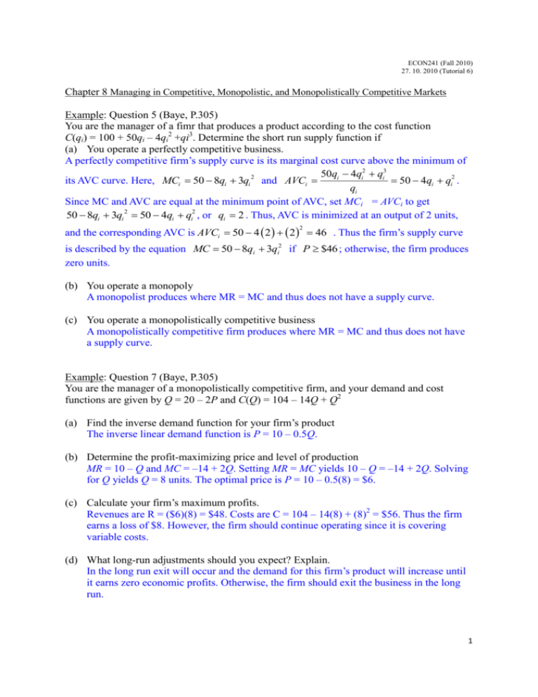
ECON241 (Fall 2010)
27. 10. 2010 (Tutorial 6)
Chapter 8 Managing in Competitive, Monopolistic, and Monopolistically Competitive Markets
Example: Question 5 (Baye, P.305)
You are the manager of a fimr that produces a product according to the cost function
C(qi) = 100 + 50qi – 4qi2 +qi3. Determine the short run supply function if
(a) You operate a perfectly competitive business.
A perfectly competitive firm’s supply curve is its marginal cost curve above the minimum of
50qi  4qi2  qi3
its AVC curve. Here, MCi  50  8qi  3qi 2 and AVCi 
 50  4qi  qi2 .
qi
Since MC and AVC are equal at the minimum point of AVC, set MCi = AVCi to get
50  8qi  3qi 2  50  4qi  qi2 , or qi  2 . Thus, AVC is minimized at an output of 2 units,
and the corresponding AVC is AVCi  50  4  2    2   46 . Thus the firm’s supply curve
2
is described by the equation MC  50  8qi  3qi2 if P  $46 ; otherwise, the firm produces
zero units.
(b) You operate a monopoly
A monopolist produces where MR = MC and thus does not have a supply curve.
(c) You operate a monopolistically competitive business
A monopolistically competitive firm produces where MR = MC and thus does not have
a supply curve.
Example: Question 7 (Baye, P.305)
You are the manager of a monopolistically competitive firm, and your demand and cost
functions are given by Q = 20 – 2P and C(Q) = 104 – 14Q + Q2
(a) Find the inverse demand function for your firm’s product
The inverse linear demand function is P = 10 – 0.5Q.
(b) Determine the profit-maximizing price and level of production
MR = 10 – Q and MC = –14 + 2Q. Setting MR = MC yields 10 – Q = –14 + 2Q. Solving
for Q yields Q = 8 units. The optimal price is P = 10 – 0.5(8) = $6.
(c) Calculate your firm’s maximum profits.
Revenues are R = ($6)(8) = $48. Costs are C = 104 – 14(8) + (8)2 = $56. Thus the firm
earns a loss of $8. However, the firm should continue operating since it is covering
variable costs.
(d) What long-run adjustments should you expect? Explain.
In the long run exit will occur and the demand for this firm’s product will increase until
it earns zero economic profits. Otherwise, the firm should exit the business in the long
run.
1
Example: Question 9 (Baye, P.306)
A monopolist’s inverse demand function is P = 100 – Q. The company produces output at two
facilities; the marginal cost of producing at facility 1 is MC1(Q1) = 4Q1, and the marginal cost
of producing at facility 2 is MC2(Q2) = 2Q2
(a) Provide the equation for the monopolist’s marginal revenue function
Since the inverse demand is P  100  Q1  Q2 , marginal revenue is
MRQ  100  2Q1  2Q2 .
(b) Determine the profit-maximizing level of output for each facility
Solving these two equations simultaneously
100  2Q1  2Q2  4Q1
100  2Q1  2Q2  2Q2
It yields Q1 = 10 and Q2 = 20.
(c) Determine the profit maximizing price
Given Q1 = 10 and Q2 = 20, P  100  10  20  $70 .
2
Chapter 9 Basic Oligopoly Models
Example: Question 3 (Baye, P. 343)
The following diagram illustrates the reaction functions and isoprofit curves for a
homogeneous-product duopoly in which each firm produces at constant marginal cost.
(a) If your rival produces 50 units of output, what is your optimal level of output?
125 units
(b) In equilibrium, how much will each firm produce in a Cournot oligopoly?
100units each
(d) How much output would be produced if the market were monopolized?
150 units
(e) Suppose you and your rival agree to collusive arrangement in which each firm produces
half of the monopoly output.
(1) What is your output under the collusive arrangement?
75 units
(2) What is your optimal output if you believe your rival will live up to the agreement?
About 112.5 units
3
Example: Lecture notes Oligopoly models P.15
Safe Ride Products markets its products in an oligopoly in which all makers of similar
products are keenly aware of what each other is doing. Safe Ride Products perceives the
demand function for its new road-emergency kit to be a kinked line with two different slopes.
Above the kink, D1: Q1 = 85 – P1 or P1 = 85 – Q1
While below the kink, D2: Q2 = 32.5 – 0.25P2 or P2 = 130 – 4Q2
The firm’s total cost, TC = 375 + 25Q + 0.6Q2
(a) Using the kinked-demand-curve model, what is the firm’s output, price and the profit at
the kink?
The kink in the firm’s demand function occurs in the intersection of the two differently
sloped segments.
D1 = Q1 = 85 – P = 130 – 4Q2 = D2  3Q = 45  Q = 15
At the kink, P = P1 = P2
P1 = 85 -15 = $70 or P2 = 130 – 4(15) = $70
 = TR – TC = 70(15) – 375 – 25(15) – 0.6(15)2 = $165
(b) Are this output, price and the profit optimal?
The output, price and profit are optimal if MR = MC
TR1 = 85Q – Q2  MR1 = 85 – 2Q = 85 – 2(15) = $55. This is the upper limit of the MR
gap.
Also, TR2 = 130Q – 4Q2  MR2 = 130 – 8Q = 130 – 8(15) = $10. This is the lower limit
of the MR gap.
Marginal cost can range from a low of $10 to a high of $55 at Q = 15 without
changing the optimal output (15 units) and price ($70)
We note that TC = 375 + 25Q + 0.6Q2 and MC = 25 + 1.2Q = 25 + 1.2(15) = $43
Since this MC falls within the gap between $10 and $55, we conclude that profit is
maximized at an optimal output of 15 units selling for $70 per unit.
(c) Graph this problem.
4