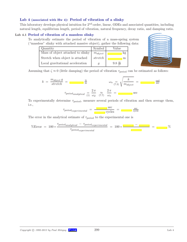
Lab 4 (associated with Hw 4): Period of vibration of a slinky
This laboratory develops physical intuition for 2nd -order, linear, ODEs and associated quantities, including
natural length, equilibrium length, period of vibration, natural frequency, decay ratio, and damping ratio.
Lab 4.1 Period of vibration of a massless slinky
To analytically estimate the period of vibration of a mass-spring system
(“massless” slinky with attached massive object), gather the following data:
Quantity
Symbol
Value
Mass of object attached to slinky mobject
kg
Stretch when object is attached
stretch
Local gravitational acceleration
m
g
9.8
m
s2
Assuming that ζ ≈ 0 (little damping) the period of vibration τperiod can be estimated as follows:
mobject g
k
N
rad
=
ωn =
=
k =
m
sec
stretch
mobject
(7.3)
τperiod analytical =
(1)
2π
ωd
≈
(7.7)
2π
=
ωn
sec
To experimentally determine τperiod , measure several periods of vibration and then average them,
i.e.,
sec
sec
=
τperiod experimental =
cycle
cycles
The error in the analytical estimate of τperiod to the experimental one is
%Error = 100 ∗
τperiod analytical − τperiod experimental
c 1992-2013 by Paul Mitiguy
Copyright τperiod experimental
299
= 100 ∗
−
=
%
Lab 4
Lab 4.2 A better model: Period of vibration of a massive slinky
The previous experiment showed how to experimentally determine the period of vibration (τperiod )
of a massive objected suspended by a “massless” slinky. To account for modeling errors associated
with the mass of the slinky, the period of vibration is recalculated with the following data:
Quantity
Mass of object attached to slinky
Symbol
mobject
Natural length of slinky (completely unstretched)
Value
kg
Ln
m
Equilibrium length of vertical slinky without attached object
LeqA
m
Equilibrium length of vertical slinky with attached object
LeqB
Local gravitational acceleration
g
m
9.8
m
s2
By using the equations which govern the static equilibrium lengths of the slinky (with and without
the attached object), one can estimate τperiod . The process consists of the following steps.
• Measure Ln , the slinky’s natural length (the slinky’s length when it is completely unstretched).
• This experiment models the slinky’s mass as a particle of mass mspring attached to the end of
the slinky. This is the mass required to stretch the slinky to LeqA . Carefully measure LeqA .
• Attach an object of known mass to the slinky. Measure LeqB (the new equilibrium length).
• Show how to use F = ma to calculate k (the slinky’s linear spring constant) and mspring .
Ln
LeqA
LeqB
k =
mspring =
mobject g
LeqB − LeqA
k
(LeqA − Ln )
g
N
m
=
=
kg
• Calculate the motion’s natural frequency ωn and τperiod analytical (the mathematically determined period of vibration).
k
rad
=
=
ωn
sec
mspring + mobject
∆
ωd
=
ωn 1 − ζ 2 ≈ ωn
(when ζ is small)
(7.7)
τperiod analytical
=
(8.1)
2π
≈
ωd
sec
• Measure τperiod experimental (the experimentally determined period of vibration) by timing
several periods of vibration and then averaging them.
τperiod experimental =
c 1992-2013 by Paul Mitiguy
Copyright 300
sec
=
cycles
sec
cycle
Lab 4
• Calculate the percentage error in the analytical determination of τperiod .
Error = 100
τperiod experimental − τperiod analytical
τperiod experimental
=
%
• Using the same data, calculate the percentage error in the analytical determination of τperiod
when mspring is assumed to be zero.
Error = 100
τperiod experimental − τperiod analytical
τperiod experimental
=
%
• The error in calculating τperiod is smaller/larger (circle one) when one assumes mspring = 0.
• Make a rough sketch that is useful for experimentally measuring the decay ratio.
decayRatio ≈
• Make a rough estimate of the damping ratio ζ. (See Homework 4.4 for details).
ζ ≈
c 1992-2013 by Paul Mitiguy
Copyright 301
Lab 4