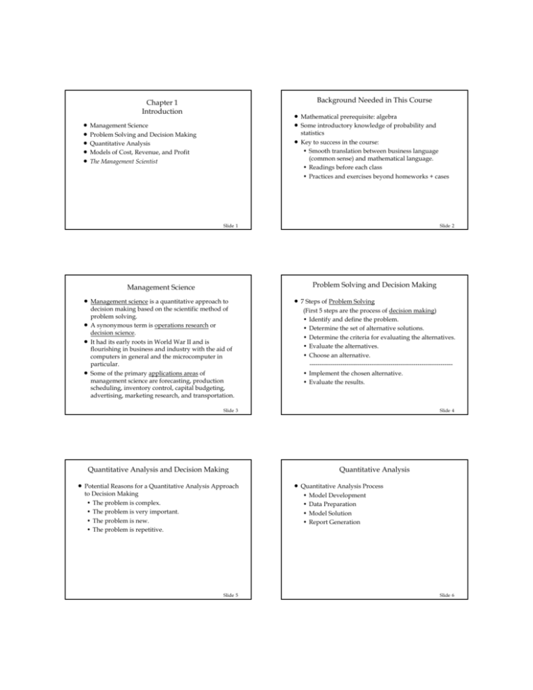
Background Needed in This Course
Chapter 1
Introduction
n
Management Science
Problem Solving and Decision Making
Quantitative Analysis
Models of Cost, Revenue, and Profit
The Management Scientist
n
n
n
n
n
n
n
Mathematical prerequisite: algebra
Some introductory knowledge of probability and
statistics
Key to success in the course:
• Smooth translation between business language
(common sense) and mathematical language.
• Readings before each class
• Practices and exercises beyond homeworks + cases
Slide 1
Slide 2
Problem Solving and Decision Making
Management Science
n
n
n
n
Management science is a quantitative approach to
decision making based on the scientific method of
problem solving.
A synonymous term is operations research or
decision science.
It had its early roots in World War II and is
flourishing in business and industry with the aid of
computers in general and the microcomputer in
particular.
Some of the primary applications areas of
management science are forecasting, production
scheduling, inventory control, capital budgeting,
advertising, marketing research, and transportation.
n
7 Steps of Problem Solving
(First 5 steps are the process of decision making)
• Identify and define the problem.
• Determine the set of alternative solutions.
• Determine the criteria for evaluating the alternatives.
• Evaluate the alternatives.
• Choose an alternative.
--------------------------------------------------------------------• Implement the chosen alternative.
• Evaluate the results.
Slide 3
Slide 4
Quantitative Analysis and Decision Making
n
Potential Reasons for a Quantitative Analysis Approach
to Decision Making
• The problem is complex.
• The problem is very important.
• The problem is new.
• The problem is repetitive.
Slide 5
Quantitative Analysis
n
Quantitative Analysis Process
• Model Development
• Data Preparation
• Model Solution
• Report Generation
Slide 6
Model Development
n
n
Mathematical Models
Models are representations of real objects or
situations.
Three forms of models are iconic, analog, and
mathematical.
• Iconic models are physical replicas (scalar
representations) of real objects.
• Analog models are physical in form, but do not
physically resemble the object being modeled.
• Mathematical models represent real world
problems through a system of mathematical
formulas and expressions based on key
assumptions, estimates, or statistical analyses.
n
n
n
Cost/benefit considerations must be made in
selecting an appropriate mathematical model.
Frequently a less complicated (and perhaps less
precise) model is more appropriate than a more
complex and accurate one due to cost and ease of
solution considerations.
The purpose, or value, of any model is that it enables
us to make inferences about the real situation by
studying and analyzing the model.
• more efficient; less time required.
• less expensive.
Slide 7
Slide 8
Mathematical Models
n
n
n
n
n
Example: Iron Works, Inc.
Mathematical models relate decision variables (or
controllable inputs) with fixed or variable parameters
(or uncontrollable inputs).
Frequently mathematical models seek to maximize or
minimize some objective function subject to constraints.
If any of the uncontrollable inputs is subject to variation
the model is said to be stochastic; otherwise the model
is said to be deterministic.
Generally, stochastic models are more difficult to
analyze.
The values of the decision variables that provide the
mathematically-best output are referred to as the
optimal solution for the model.
Iron Works, Inc. (IWI) manufactures two products
made from steel and just received this month's
allocation of b pounds of steel. It takes a1 pounds of
steel to make a unit of product 1 and it takes a2 pounds
of steel to make a unit of product 2.
Let x1 and x2 denote this month's production level
of product 1 and product 2, respectively. Denote by p1
and p2 the unit profits for products 1 and 2,
respectively.
The manufacturer has a contract calling for at least
m units of product 1 this month. The firm's facilities are
such that at most u units of product 2 may be produced
monthly.
Slide 9
Slide 10
Example: Iron Works, Inc.
n
Example: Iron Works, Inc.
Mathematical Model
• The total monthly profit =
(profit per unit of product 1)
x (monthly production of product 1)
+ (profit per unit of product 2)
x (monthly production of product 2)
= p1x1 + p2x2
We want to maximize total monthly profit:
Max p1x1 + p2x2
n
Slide 11
Mathematical Model (continued)
• The total amount of steel used during monthly
production =
(steel required per unit of product 1)
x (monthly production of product 1)
+ (steel required per unit of product 2)
x (monthly production of product 2)
= a1x1 + a2x2
This quantity must be less than or equal to the
allocated b pounds of steel:
a1x1 + a2x2 < b
Slide 12
Example: Iron Works, Inc.
n
Example: Iron Works, Inc.
Mathematical Model (continued)
• The monthly production level of product 1 must be
greater than or equal to m:
x1 > m
• The monthly production level of product 2 must be
less than or equal to u:
x2 < u
• However, the production level for product 2 cannot
be negative:
x2 > 0
n
Mathematical Model Summary
Max p1x1 + p2x2
s.t.
a1x1 + a2x2 <
>
x1
x2 <
x2 >
b
m
u
0
Slide 13
Slide 14
Example: Iron Works, Inc.
n
n
Example: Iron Works, Inc.
Question:
Suppose b = 2000, a1 = 2, a2 = 3, m = 60, u = 720, p1 =
100, p2 = 200. Rewrite the model with these specific
values for the uncontrollable inputs.
Answer:
Substituting, the model is:
Max 100x1 + 200x2
s.t.
2x1 + 3x2 < 2000
> 60
x1
x2 < 720
0
x2 >
n
n
Question:
The optimal solution to the current model is x1 = 60
and x2 = 626 2/3 [after using the Management Scientist].
If the product were engines, explain why this is not a
true optimal solution for the "real-life" problem.
Answer:
One cannot produce and sell 2/3 of an engine.
Thus the problem is further restricted by the fact that
both x1 and x2 must be integers. They could remain
fractions if it is assumed these fractions are work in
progress to be completed the next month.
Slide 15
Slide 16
The Management Scientist
n
The Management Scientist
Major Elements
• Top Level Menu
• Problem Selection Menu
• Data Input
• Problem Disposition Menu
• Solution and Output Information
• Data Editing
• Saving, Retrieving, and/or Deleting Problems
n
1
2
3
4
5
6
Slide 17
Top Level Menu
THE MANAGEMENT SCIENTIST
Top Level Menu
Linear Programming
7 PERT/CPM
Transportation
8 Inventory Models
Assignment
9 Waiting Lines
Integer Linear Programming
10 Decision Analysis
Shortest Route
11 Forecasting
Minimal Spanning Tree
12 Markov Processes
13 EXIT PROGRAM
Slide 18
The Management Scientist
n
The Management Scientist
Problem Selection Menu
n
PROBLEM SELECTION MENU
Choices
1 Create a New Problem
2 Retrieve a Previously Saved Problem
3 Continue with the Current Problem
4 Delete a Previously Saved Problem
5 Return to the Top Level Menu
Problem Disposition Menu
PROBLEM DISPOSITION MENU
Choices
1 Solve the Problem
2 Save the Problem
3 Display/Edit the Problem
4 Return to the Problem Selection Menu
Slide 19
Breakeven Analysis
Slide 20
The End of Chapter 1
Fixed costs (cf) - costs that remain constant regardless of
number of units produced
Variable cost (cv) - unit cost of product
Total variable cost (v cv) - function of volume (v) and
variable per-unit cost
Total cost (TC) - total fixed cost plus total variable cost
Profit(Z) - difference between total revenue vp (p=price)
and total cost:
Z = v p - cf – v cv
The break-even point is that volume at which total
revenue equals total cost and profit is zero:
V = cf/(p-cv)
Slide 21
Slide 22
Self Quiz
n
n
Self Quiz
Algebra Basics: Solve for x1 and x2 in the following
equations
4x1 - x2 = 12
x1+ x2 = 4
Statistics Basics: Suppose z is a standard normal
variable (with mean 0 and standard deviation of 1).
• What is the probability that z is less than z0=1?
• What is the probability that z is greater than z0=1?
Slide 23
The price of a particular stock listed in NYSE is fluctuating
up and down from one transaction to the next
according to the following probability distribution.
Price
Change Probability
-3/8
.08
-1/4
.04
-1/8
.16
0
.40
+1/8
.20
+1/4
.06
+3/8
.04
+1/2
.02
TOTAL 1.00
Q: What is the cumulative probability that the
price change is less than and equal to +1/4?
Q: What is the expected amount of price
change (per transaction)?
Slide 24