Proceedings of the Twenty-Eighth AAAI Conference on Artificial Intelligence
Large-Scale Optimistic Adaptive Submodularity
Victor Gabillon
Branislav Kveton
Zheng Wen
INRIA Lille - team SequeL
Villeneuve d’Ascq, France
victor.gabillon@inria.fr
Technicolor Labs
Palo Alto, CA
branislav.kveton@technicolor.com
Electrical Engineering Department
Stanford University
zhengwen@stanford.edu
Brian Eriksson
S. Muthukrishnan
Technicolor Labs
Palo Alto, CA
brian.eriksson@technicolor.com
Department of Computer Science
Rutgers
muthu@cs.rutgers.edu
Abstract
the items and their states are the sensors and measurements,
respectively; and the objective is to gather most informative
data.
In many situations, the model of the problem is unknown
and can be only learned while solving the problem. In preference elicitation, for example, it is hard to say how useful
the questions are before they are asked. Recently, Gabillon
et al. (2013) proposed a learning algorithm for solving such
problems, learning how to maximize an adaptive submodular function while maximizing it. A major limitation of this
solution is that its regret grows linearly with the number of
items L. In practice, L is large and the solution of Gabillon
et al. (2013) becomes impractical. In this work, we address
the problem of scalable learning in adaptive submodularity.
In many practical problems, items have features and their
states are distributed similarly when the features are similar.
In preference elicitation, for instance, similar questions are
likely to have similar answers. In a sensor network, nearby
sensors may record similar data. In this work, we show how
to leverage this structure to learn the model of our problem
more efficiently. More specifically, we assume that the state
of each item is distributed according to a parametric model,
which is conditioned on the features of the item. Our objective is to learn the parameters of this model.
Our problem is challenging for several reasons. First, the
model of the problem is not known. Second, the state space
is exponential in the number of items L. Finally, the state is
only partially observable. In a sense, our problem combines
the challenges of large-scale reinforcement learning (Sutton
and Barto 1998) and partially-observable Markov decision
processes (POMDPs) (Sondik 1971), each of which is considered to be a hard problem. Therefore, it is unclear if our
problem can be solved efficiently.
We make three contributions. First, we present a scalable
algorithm for learning how to maximize adaptive submodular functions. The key structural assumption in our work is
that the state of each item is distributed according to a generalized linear model (GLM) (McCullagh and Nelder 1989),
which is conditioned on the features of the item. Our algorithm is conceptually simple and easy to implement.
Maximization of submodular functions has wide applications
in artificial intelligence and machine learning. In this paper,
we propose a scalable learning algorithm for maximizing an
adaptive submodular function. The key structural assumption
in our solution is that the state of each item is distributed according to a generalized linear model, which is conditioned
on the feature vector of the item. Our objective is to learn the
parameters of this model. We analyze the performance of our
algorithm, and show that its regret is polylogarithmic in time
and quadratic in the number of features. Finally, we evaluate
our solution on two problems, preference elicitation and face
detection, and show that high-quality policies can be learned
sample efficiently.
1
Introduction
Submodularity (Nemhauser, Wolsey, and Fisher 1978) has
many applications in machine learning and artificial intelligence, such as influence maximization (Kempe, Kleinberg,
and Tardos 2003), recommendations (Guillory and Bilmes
2011; Bhamidipati, Kveton, and Muthukrishnan 2013), and
sensor placement (Krause, Singh, and Guestrin 2008). All
of these problems can be formulated as maximizing a submodular function on a set of items. Nemhauser et al. (1978)
showed that this problem can be solved near optimally by a
greedy algorithm. The algorithm is conceptually simple and
widely used in practice.
Adaptive submodularity (Golovin and Krause 2011) is a
framework for maximizing adaptive submodular functions.
In this framework, each item has a state and this state is revealed when the item is chosen. The objective is to choose
adaptively a set of items that maximize the expected return.
Adaptive submodularity is suitable for modeling interactive
decision problems, such as preference elicitation and active
sensing. In preference elicitation, the items and their states
are the questions and answers, respectively; and the goal is
to elicit the most informative user profile. In active sensing,
c 2014, Association for the Advancement of Artificial
Copyright Intelligence (www.aaai.org). All rights reserved.
1816
policy in state φ, πk (φ), is the collection of the first k items
chosen by policy π. The policy is defined recursively as:
πk (φ) = πk−1 (φ) ∪ π[k] (φ)
Second, we prove an upper bound on the expected cumulative regret of our algorithm. The bound is polylogarithmic
in time and quadratic in the number of features, as in GLM
bandits (Filippi et al. 2010). It also reflects the shape of the
optimized submodular function, as in Gabillon et al. (2013).
In summary, we bring together the concepts of bandits and
submodularity in a natural way, which allows to analyze the
resulting problem.
Finally, we evaluate our solution on two real-world problems. The first problem is learning of an adaptive policy for
movie recommendation. The second problem is learning of
an adaptive face detector. In both domains, we demonstrate
that high-quality policies can be learned fast, from just several hundred interactions with the environment.
2
π[k] (φ) = π(φhπk−1 (φ)i)
where π[k] (φ) is the k-th item chosen by policy π in state φ.
The optimal K-step policy satisfies:
π ∗ = arg maxπ Eφ [f (πK (φ), φ)] .
Adaptive submodularity (Golovin and Krause 2011) can be
viewed as a special form of a partially-observable Markov
decision process (POMDP) (Sondik 1971). The state of this
process φ is initially unknown and is revealed by actions A.
The goal is to maximize a submodular function f (A, φ) of
the state φ and actions A.
Formally, we maximize a function of the form:
L
Definition 1. Function f is adaptive submodular if:
Eφ [ f (A ∪ {i} , φ) − f (A, φ) | φ ∼ yA ]
≥ Eφ [ f (B ∪ {i} , φ) − f (B, φ) | φ ∼ yB ]
for all items i ∈ I \ B and observations yB yA such that
A = dom(yA ) and B = dom(yB ).
(1)
Definition 2. Function f is adaptive monotonic if:
I
where I = {1, . . . , L} is a set of L items and 2 is its power
set. The first argument of f is a set of chosen items A ⊆ I.
L
The second argument is the state φ ∈ {−1, 1} of all items.
The i-th entry of φ, φ[i], is the state of item i. The state φ is
drawn i.i.d. from some probability distribution P (Φ). The
return for choosing items A in state φ is f (A, φ). Without
loss of generality, we assume that f (∅, φ) = 0 in all states
φ. The state is only partially observed. An observation is a
L
vector y ∈ {−1, 0, 1} such that its non-zero entries are the
observed states of items. More specifically, we say that y is
an observation of state φ, and write φ ∼ y, if y[i] = φ[i] in
all non-zero entries of y. The state φ can be also viewed as
a realization of y. We denote by dom(y) = {i : y[i] 6= 0}
the set of observed items in y and by φhAi the observation
of items A in state φ. We assume that the observations are
partially ordered and write y0 y if y0 [i] = y[i] in all nonzero entries of y, y0 is a more specific observation than y.
We illustrate our notation on a simple example. Let φ =
(1, 1, −1) be a state, and y1 = (1, 0, 0) and y2 = (1, 0, −1)
be observations. Then all of the following claims are true:
φ ∼ y1 ,
y2 y1 ,
φ ∼ y2 , dom(y2 ) = {1, 3} ,
Eφ [ f (A ∪ {i} , φ) − f (A, φ) | φ ∼ yA ] ≥ 0
for all items i ∈ I \ A and observations yA such that A =
dom(yA ).
In other words, the expected gain of choosing items is nonnegative and does not increase as the observations become
more specific. Let:
π g (y) = arg max gi (y)
be the greedy policy for maximizing f and:
gi (y) = Eφ [f (dom(y) ∪ {i} , φ) −
f (dom(y) , φ) | φ ∼ y]
(6)
denote the expected gain of choosing item i after observing
y. Then π g is a (1 − 1/e)-approximation to π ∗ :
g
∗
Eφ [f (πK
(φ), φ)] ≥ (1 − 1/e)Eφ [f (πK
(φ), φ)]
(7)
when the function f is adaptive submodular and monotonic
(Golovin and Krause 2011).
The greedy policy π g cannot be computed when the distribution P (Φ) is unknown. Gabillon et al. (2013) proposed
a bandit algorithm for such problems, Optimistic Adaptive
Submodular Maximization (OASM), that learns P (Φ) by interacting with the environment. A major assumption in this
work is that P (Φ) is a product of L Bernoulli distributions,
one for the state of each item. In this setting, the problem of
learning P (Φ) reduces to learning L parameters, one mean
pi for each distribution. Unfortunately, the expected cumulative regret of OASM grows linearly with L. As a result, the
method is impractical when L is large.
Our goal is to maximize the expected value of f by adaptively choosing K items. The items are chosen sequentially
according to some policy π and we observe the state of each
chosen item. A policy:
L
(5)
i∈I\dom(y)
φh{1, 3}i = y2 ,
φhdom(y1 )i = y1 .
π : {−1, 0, 1} → I
(4)
It is NP-hard to compute the policy π ∗ (Golovin and Krause
2011). However, near-optimal policies can be computed efficiently when the optimized function has a diminishing return property. Specifically, we require that the function f is
adaptive submodular and monotonic.
Adaptive Submodularity and Learning
f : 2I × {−1, 1} → R,
(3)
π0 (φ) = ∅,
(2)
is a function from observations y to items. The observation
represents our past decisions and their outcomes. A k-step
1817
3
The difference between the expected returns of π g and π t is
the expected cumulative regret of π t :
" n
#
X
Rt (φt ) ,
R(n) = Eφ1 ,...,φn
(13)
Optimistic Adaptive Submodularity with
Generalized Linear Models
In this work, we propose a learning algorithm whose regret
does not depend on the number of items L. We assume that
each item is associated with a feature vector xi and that the
states of the item are distributed conditionally on xi .
3.1
t=1
g
t
where Rt (φt ) = f (πK
(φt ), φt ) − f (πK
(φt ), φt ). In maxg
imum coverage problems, the policy π is a good surrogate
for π ∗ because it is a (1 − 1/e)-approximation to π ∗ .
Model
The feature vector of item i is a d-dimensional column vector xi ∈ Rd such that kxi k2 ≤ c. To simplify our notation,
we define x = (x1 , . . . , xL ) ∈ RdL , a vector of all feature
vectors. We assume that the vector x is known and does not
change with time t.
The distribution of states is factored as:
P (Φ = φ) =
L
Y
1{φ[i]=−1}
pi (x)1{φ[i]=1} (1 − pi (x))
3.2
, (8)
i=1
where pi (x) is the probability that item i is in state 1. The
probability pi (x) is unknown and we want to learn it. Since
the state of each item i is binary, the dependency on xi can
be naturally modeled using logistic regression:
pi (x) = P (φ[i] = 1 | xi ) = µ(xTi θ∗ ),
Algorithm
Our learning algorithm has two main parts. First, at the beginning of each episode, we estimate θ∗ from past observation using regression. Second, in each step of each episode,
we behave optimistically and greedily choose the item with
the highest upper confidence bound on its gain. More pret
cisely, at step k of episode t, we select item π[k]
(φt ), which
t
t
we abbreviate as π[k]
, and then observe its state φt [π[k]
].
The pseudo-code of our method is given in Algorithm 1.
The parameters θ∗ are estimated as follows. First, we compute the maximum-likelihood estimate θ̂t of θ∗ . By definition, θ̂t maximizes the regularized log-likelihood:
K n
t−1 X
o
X
s
s (x)) +
1 φs [π[k]
] = 1 log(pπ[k]
(9)
where µ(u) = 1/(1 + e−u ) is a logistic function, θ∗ ∈ Θ is
a column vector of learned parameters such that kθ∗ k2 ≤ S,
and Θ ⊂ Rd is a compact and convex space.
Our choice of µ is motivated by the fact that the states of
all items in our problem are binary. However, note that this
assumption is only for simplicity of exposition. Our results
apply to any generalized linear model. In fact, we only need
to assume that µ is zµ -Lipschitz continuous, increasing, and
continuously differentiable such that cµ = inf µ̇(xTi θ) > 0.
s=1 k=1
n
o
1
2
s
s (x))
1 φs [π[k]
] = −1 log(1 − pπ[k]
− λ kθk2
2
"
!
K
t−1 X
n
o
s (x)
X
pπ[k]
s
1 φs [π[k] ] = 1 log
=
+
s (x)
1 − pπ[k]
s=1 k=1
#
1
2
s (x))
log(1 − pπ[k]
− λ kθk2
2
t−1 X
K n
o
X
s
=
1 φs [π[k]
] = 1 xTπs θ −
θ∈Θ,i
With our model in mind, we rewrite the expected gain of
choosing item i (Equation 6) as:
[k]
gi (y) = pi (x)ḡi (y),
s=1 k=1
(10)
log 1 + e
where:
ḡi (y) = Eφ [f (dom(y) ∪ {i} , φ) −
f (dom(y) , φ) | φ ∼ y, φ[i] = 1]
(11)
xT
πs θ
[k]
1
2
− λ kθk2 ,
2
(14)
which is concave in θ. Upon differentiating, we obtain that
θ̂t is a unique solution to:
t−1 X
K n
o
X
s
1 φs [π[k]
]=1 −
(15)
is the expected gain of choosing item i in state 1.1 In many
problems of interest, the gain ḡi (y) is only a function of y
and i (Gabillon et al. 2013), and therefore can be computed
without knowing P (Φ).
Our learning problem is episodic. In episode t, we adaptively select K items according to some policy π t , which is
episode dependent. The state in episode t is φt . The quality
of π t is measured by its expected cumulative K-step return:
" n
#
X
t
Eφ1 ,...,φn
f (πK (φt ), φt ) .
(12)
s=1 k=1
T
µ xπ s
[k]
s
θ xπ[k]
− λθ = 0.
Second, to solve a technical detail in our proof, we need to
guarantee that our solution is in Θ. Therefore, we project θ̂t
into Θ. For this purpose, we define an invertible function:
ht : θ 7→
t=1
t−1 X
K
X
s
µ xTπs θ xπ[k]
+ λθ
[k]
(16)
s=1 k=1
1
For simplicity of exposition, we assume that the expected gain
of choosing item i in state −1 is zero. Our work can be straightforwardly generalized to the problems where this gain is non-zero.
and let:
θ̃t = arg min ht (θ) − ht (θ̂t )M −1
θ∈Θ
1818
t
(17)
Algorithm 1 LinOASM: Optimistic adaptive submodularity
with a generalized linear model.
be the resulting projection, where:
Mt =
t−1 X
K
X
T
s x s
+ λI
xπ[k]
π
[k]
(18)
Input:
Feature vectors x1 , . . . , xL
Regularization parameter λ
s=1 k=1
s
is the Gram matrix of all feature vectors xπ[k]
up to episode
t and I is a d × d identity matrix. We add the regularization
term λI to guarantee that Mt is invertible. The influence of
this term vanishes as the number of episodes increases.
At each step k, we compute the index of each item i:
h
i
i
µ(xTi θ̃t ) + βk,t
(δ) ḡi (y).
(19)
for all t = 1, . . . , n do
Estimate θ̃t based on Equations 15 and 17
A←∅
for all k = 1, . . . , K do
y ← φt hAi h
i
i
j ← arg max µ(xTi θ̃t ) + βk,t
(δ) ḡi (y)
The term:
i
βk,t
(δ) = ρk,t (δ)kxi kM −1
t
i∈I\A
(20)
A ← A ∪ {j}
end for
end for
is the radius of the confidence interval around µ(xTi θ̃t ), the
estimate of the probabilityqthat item i is in state 1. The norm
is defined as kukM −1 = uT Mt−1 u. Therefore, kxi kM −1
t
t
can be interpreted as the variance of our regressor at item i.
The quantity ρk,t (δ) is a slowly increasing function in t and
k, which is defined as:
4zµ
(3 + 2 log (1 + 2c2 /λ)) ×
(21)
ρk,t (δ) =
cµ
hp
i
1
2d log(tK + k) log(2(tK + k)nK/δ) + λ 2 S .
i
(δ) with
Based on this setting, µ(xTi θ∗ ) − µ(xTi θ̃t ) ≤ βk,t
probability of at least 1 − δ, simultaneously for all episodes
t ≤ n and steps.
After we compute all indices, we select the item with the
highest upper confidence bound. The indices enforce exploration of items that have not been chosen very often. As the
number of past episodes increases, we get a better estimate
of θ∗ , all confidence intervals kxi kM −1 shrink, and we start
t
exploiting best items.
LinOASM is a greedy method. Therefore, our policies can
be computed very fast. In particular, the time complexity of
LinOASM at step k is O(L), because we need to recompute
the index of each item (Equation 19). Moreover, estimation
of θ̂t (Equation 15) is straightforward, because this is just a
regression problem. Finally, our solutions are guaranteed to
converge to π g . This claim is proved in the next section.
3.3
the set of observations where item i is suboptimal at step k.
The hardness of discriminating items i and π g (y) in context
y is measured by the gap between the expected gains of the
items:
∆i (y) = gπg (y) (y) − gi (y).
Our main result is presented below.
Theorem 1. Let λ ≥ d2 . Then the expected cumulative regret of LinOASM is bounded as:
R(n) ≤
K
X
Gk (`k + nδ),
k=1
|
{z
O(log3 n)
}
where Gk = (K − k + 1) max max gi (y) is an upper bound
y∈Yk
i
on the expected gain of π g from step k forward and:
`k = dd/Ke + 8dρ2K,n (δ) ×
2
ḡi2 (y)
c nK
max max 2
log
i y∈Yk,i ∆i (y)
λ
is the number of episodes after which no item is likely to be
chosen suboptimally at step k.
Analysis
Proof. The proof of our claim is in Appendix. It consists of
three main parts. First, we associate the regret in episode t
with the first step where π t selects a different item from π g .
Second, we bound the expected regret in each episode t by
the probability of deviating from the policy π g at step k and
an upper bound on the associated loss Gk , which is derived
based on the submodularity of f . This part of the analysis is
motivated by the work of Gabillon et al. (2013). Finally, we
bound the expected number of suboptimally selected items
based on a high-probability upper bound on the cumulative
regret of our regressor. This part of the proof borrows ideas
from Filippi et al. (2010).
In this section, we prove a gap-dependent bound on the expected cumulative regret of LinOASM. Our analysis is based
on counting the number of times when the policy π t selects
a different item from the policy π g at step k. Therefore, we
define several variables that allow us to describe the state of
our problem at this step. We denote by:
[
Yk (π) =
{φhπk−1 (φ)i}
(22)
φ
the set of all possible observations after policy π is applied
for k − 1 steps. The observations associated with the policy
π g are denoted by Yk = Yk (π g ). We denote by:
Yk,i = Yk ∩ {y : i 6= π g (y)}
(24)
The scalar δ is a parameter of our learning algorithm. For a
given number of episodes n, it should be set as δ = 1/n. In
(23)
1819
Symbol
n
K
d
xi
c
θ∗
S
Θ
µ
zµ
cµ
λ
θ̂t
θ̃t
Mt
i
βk,t
ρk,t
1−δ
Description
Number of episodes
Number of steps in each episode
Number of features
Feature vector of item i
Upper bound on kxi k2
Unknown parameter vector
Upper bound on kθ∗ k2
Compact and convex space such that θ∗ ∈ Θ
Mean function
Lipschitz constant of µ
Lower bound on µ̇
Regularization parameter
ML estimate of θ∗ in episode t
Estimate of θ∗ in episode t
Gram matrix in episode t
Confidence radius for µ(xTi θ̃t )
Slowly increasing function in t and k
Probability that our regret bound holds
of LinOASM and π g is the loss due to our modeling assumptions, one of which is Equation 8.
4
LinOASM is evaluated on two real-world problems. The first
problem is learning of a policy for movie recommendation.
The problem is motivated by a movie rating game on Netflix
(net 2013), where the users are asked to rate a set of movies
to improve their profile. The second problem is learning of
an adaptive face detection policy. The problem is motivated
by a range of adaptive sensing problems in computer vision
(Tarabanis, Allen, and Tsai 1995; Butko and Movellan 2009;
Vijayanarasimhan and Kapoor 2010). In all of these problems, the computational resources of the algorithm are limited and as a result the algorithm must behave intelligently.
Both of our problems are set up such that we can showcase
the benefits of submodularity.
All policies are evaluated by the expected per-step return
in n episodes, the expected cumulative return in n episodes
divided by n. The parameterization of LinOASM suggested
by our analysis (Section 3.3) is too conservative in practice,
as in GLM bandits (Filippi et al. 2010). In our experiments,
we choose λ = 1 and ρk,t (δ) = 0.1 log(tK + k). At these
values, LinOASM performs well and is not sensitive to small
perturbations of the parameters. Note that ρk,t (δ) is chosen
such that it depends on t and k at the same rate as in Equation 21.
LinOASM is compared to three baselines. The first baseline is OASM (Gabillon et al. 2013), a learning algorithm for
adaptive submodular maximization that does not utilize the
features of items. The second baseline is an ε-greedy policy
with the same linear generalization model as LinOASM. We
set ε to 0.1. This method can be viewed as a naive solution
to our problem that leverages its structure. Finally, the third
baseline is π g (Equation 5). The policy π g knows P (Φ) and
does not assume any structure. Therefore, π g can be viewed
as an upper bound on the performance of LinOASM.
Table 1: Summary of our GLM bandit notation.
this case, our regret bound is polylogarithmic in n, through
the terms `k . This dependency on n is the same as in GLM
bandits (Filippi et al. 2010).
Our regret bound also captures the submodular character
of our problem. Specifically, because f is adaptive submodular, the upper bound on the expected gain of the policy π g
from step k forward, Gk , decreases as k increases. Consequently, earlier deviations from the policy π g are penalized
more than later ones.
Remarkably, our bound is polynomial in all constants of
interest. More specifically, it is linear in K and quadratic in
the number of features d. This is a significant improvement
over Gabillon et al. (2013), whose regret bound is linear in
the number of items L. In practice, d is often much smaller
than L, and we expect significant speedups in learning over
OASM (Gabillon et al. 2013).
The regularization parameter λ is problem specific. Note
that our bound is linear in λ, through the dependency on the
term ρ2K,n (δ) (Equation 21).
3.4
Experiments
4.1
Preference Elicitation
In the first experiment, we learn a policy for recommending
movies. Our learning problem is episodic. In each episode,
we adaptively show K movies to a user. The user may like
or dislike each of the movies. Our objective is to maximize
the expected number of movies that we can recommend to
the user at the end of each episode, movies that are similar
to the movies that the user likes.
We experiment with 6k users and 500 most rated movies
from the MovieLens dataset (Lam and Herlocker 2013). The
movie preferences of any user j are represented by a vector
L
φj ∈ {−1, 1} such that φj [i] = 1 if the user likes movie i
and φj [i] = −1 otherwise. All movie preference vectors φj
are estimated from historical ratings of the users using lowrank matrix factorization (Koren, Bell, and Volinsky 2009),
a standard approach in collaborative filtering. In particular,
we factor the user-item rating matrix as M ≈ U X T , where
U is the user matrix, X is the item matrix, and the number
of latent factors is d = 10. Based on our model, user j rates
movie i as rj,i = huj , xi i, where uj and xi are the j-th row
Independence Assumption
Our independence assumption (Equation 8) allows us to develop a conceptually simple learning algorithm that can be
analyzed. In practice, the assumption may be violated. This
issue can be addressed in two ways. First, the ground set I
is reduced to the items whose states are distributed independently. This is a domain-specific preprocessing step, which
is in a sense equivalent to feature selection. In this case, we
can guarantee that LinOASM converges to the greedy policy
π g on the reduced set I. Second, LinOASM is applied to the
problem even if the states of items are not distributed independently. In this case, LinOASM converges to some suboptimal solution.
In our experiments, the states of items are not distributed
independently. The difference between the expected returns
1820
Preference elicitation
Person 2845
Person 4870
Person 1269
Person 5022
Person 2845
Person 4870
Person 1269
Person 5022
LinOASM
80
70
60
50
Policy πg
LinOASM
OASM
ε−greedy
40
30
20
0
10
1
10
2
10
Episode n
OASM
Expected per−step return
90
3
10
(a)
(b)
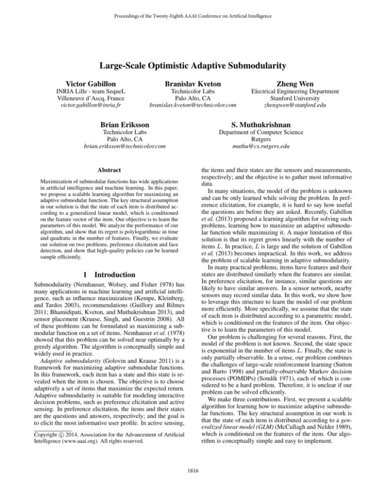
Figure 1: a. The expected per-step return of four preference elicitation policies up to episode n = 3k. b. Visualization of the
OASM and LinOASM policies in episode n = 100. The black dots are liked movies, projected on the first two components of the
latent space. The colored dots are liked movies that are similar to at least one queried movie i ∈ A that is liked.
of U and the i-th row of X, respectively. We set φj [i] to 1 if
movie i is rated highly by user j, rj,i > 4.
We say that movies i1 and i2 are similar if they are close
in the item space, kxi1 − xi2 k2 ≤ 0.2. We choose this similarity measure because it implies that the ratings of similar
movies are similar. More precisely, the L2 -norm of the user
factors in our dataset is bounded by 5 and therefore:
|rj,i1 − rj,i2 | ≤ kuj k2 kxi1 − xi2 k2 ≤ 5 · 0.2.
P (Φ) is factored (Equation 8). This is not true in our problem. As a result, LinOASM learns only an approximation of
P (Φ) and is not guaranteed to converge to π g .
We visualize our solutions in Figure 1b. LinOASM clearly
covers more liked movies than OASM. Therefore, we expect
that LinOASM would perform significantly better in practice
than OASM.
(25)
4.2
In turn, similar movies are liked similarly.
The return f (A, φ) for asking a user φ questions A is the
sum of the returns f` (A, φ), one for each movie `:
f (A, φ) =
500
X
f` (A, φ)
Adaptive Face Detection
In the second experiment, we learn a policy for face detection. Our learning problem is episodic. In each episode, we
adaptively sense K regions of an image. Our objective is to
maximize the sensed area that contains faces.
We experiment with 3k labeled images of faces from the
GENKI-SZSL dataset (UCSD 2013). Each image is resized
to 100 × 100 pixels and divided into 81 overlapping sensing
regions, which are centered at pixels:
(26)
`=1
f` (A, φ) = 0.11{∃i ∈ A : kx` − xi k2 ≤ 0.2} +
0.91{∃i ∈ A : kx` − xi k2 ≤ 0.2, φ[i] = 1} .
(u, v) ∈ {10, . . . , 90} × {10, . . . , 90} .
The return for movie ` is 1 if the movie is similar to at least
one liked movie i. The return is 0.1 if ` is similar to at least
one movie i but none of these movies are liked. Otherwise,
the return is zero. The function f (A, φ) is maximized when
A is a diverse set of liked movies. It is submodular in A for
all φ and therefore adaptive submodular when all entries of
φ are distributed independently.
The features of movie i are xi . The number of features is
d = 10. Our goal is to learn how the latent factors correlate
with liked movies. We set K to 5.
Our results are reported in Figure 1a. We observe several
trends. First, LinOASM outperforms OASM by a huge margin.
In particular, the expected return of OASM after 3k episodes
is around 50, which is comparable to the return of LinOASM
in 10 episodes. So LinOASM learns more than two orders of
magnitude faster than OASM. Second, LinOASM outperforms
the ε-greedy policy. Finally, note that the expected return of
LinOASM after 3k episodes is much lower than the return of
the policy π g . This gap is due to our modeling assumptions.
Specifically, LinOASM makes a simplifying assumption that
(27)
We assume that all regions are twenty pixels wide and high.
Several examples of the regions are in Figure 2b. The state
of a region is 1 if at least a quarter of its pixels covers a face
and −1 otherwise. Each image in our dataset is represented
81
by a vector φ ∈ {−1, 1} , which describes the states of all
regions in the image.
The return f (A, φ) for choosing regions A in image φ is
the average of the returns f` (A, φ), one for each pixel `:
f (A, φ) = E` [f` (A, φ)]
(28)
f` (A, φ) = 0.11{∃i ∈ A : region i covers `} +
0.91{∃i ∈ A : region i covers `, φ[i] = 1} .
The return for pixel ` is 1 if this pixel is covered by at least
one region i with a face. The return is 0.1 if ` is covered by
at least one region i but none of these regions contain faces.
The function f (A, φ) is maximized when A is a set of nonoverlapping regions with faces. It is submodular in A for all
states φ and therefore adaptive submodular when all entries
of φ are distributed independently.
1821
Face detection
Person 105
Person 90
Person 15
Person 174
Person 105
Person 90
Person 15
LinOASM
Person 174
0.18
0.16
0.14
Policy πg
LinOASM
OASM
ε−greedy
0.12
0.1
0.08
0
10
1
10
2
10
Episode n
OASM
Expected per−step return
0.2
3
10
(a)
(b)
Figure 2: a. The expected per-step return of four face detection policies up to episode n = 3k. b. Visualization of the OASM and
LinOASM policies in episode n = 100. The colored rectangles are the regions sensed by the policies.
The features of the region summarize the position of the
region in the image. Specifically, let region i be centered at
(u, v). Then its feature vector is:


k(u, v) − (50, 50)k2
 max {u − 50, 0} 


(29)
xi =  max {50 − u, 0}  .
 max {v − 50, 0} 
max {50 − v, 0}
Our work is also related to Yue and Guestrin (2011). Yue
and Guestrin (2011) propose a bandit algorithm that learns
how to maximize a submodular function, where the gain of
the item is a linear function of its features. The main difference in our work is that our maximization problem is adaptive. The best adaptive policy is often much better than the
best non-adaptive policy (Golovin and Krause 2011), but it
is also harder to learn. In particular, the adaptive policy is a
decision tree while the non-adaptive policy is a set of items.
In this paper, we address the harder of the two problems and
demonstrate that it can be solved at scale.
The first feature is the Euclidean distance from the center of
the image. The remaining four features are two vertical and
two horizontal distances from the center. These features are
motivated by the fact that we expect most faces close to the
center. We set K to 7.
Our results are reported in Figure 2a. We observe similar
trends to those in Section 4.1. Specifically, LinOASM learns
two orders of magnitude faster than OASM. We visualize our
solutions in Figure 2b. LinOASM clearly covers more facial
regions than OASM.
5
6
Conclusions
In this work, we study the problem of learning how to maximize adaptive submodular functions. We assume that each
item is associated with a feature vector and that the state of
the item is distributed conditionally on its features. We propose a learning algorithm that leverages this structure, and
show that its regret is polylogarithmic in time and quadratic
in the number of features. Our solution is evaluated on two
problems and we demonstrate that high-quality policies can
be learned sample efficiently. Submodularity is common in
practice and we believe that our method can solve many interesting active learning problems, such as learning policies
for near-optimal viral marketing in social networks (Kempe,
Kleinberg, and Tardos 2003).
Our method and its analysis can be easily generalized to
the setting where the feature vectors change with time (Filippi 2010). This generalization could be of interest in many
applications. For instance, the features in our face detection
problem (Section 4.2) could then depend on the content of
the image and be more informative.
Adaptive submodularity can be viewed as a special form
of POMDPs (Section 2). Therefore, it is only natural to ask
if some POMDP solver (Pineau, Gordon, and Thrun 2003)
could solve the problems in our experimental section as efficiently as LinOASM. We believe that this is unlikely. First,
the number of states in our problems is huge, 281 and 2500 ,
far out of reach of the state-of-the-art solvers. Second, note
that we learn the model of the problem, not just a policy for
Related Work
Golovin and Krause (2011) proposed adaptive submodularity, a framework for maximizing adaptive submodular functions. Wen et al. (2013) proposed a learning algorithm for a
special class of adaptive submodularity, adaptive minimum
set cover, where exploration is not necessary. The first bandit algorithm for adaptive submodularity was proposed and
analyzed by Gabillon et al. (2013). Unfortunately, this solution does not scale to large problems. In this work, we build
on the idea of Gabillon et al. (2013) and propose a scalable
learning algorithm for adaptive submodularity.
The key assumption in our paper is that the state of each
item is distributed according to a generalized linear model,
which is conditioned on the features of the item. Our generalization model is the same as in GLM bandits (Filippi et al.
2010), and both our approach and its analysis are motivated
by recent work on linear bandits, such as Dani et al. (2008)
and Abbasi-Yadkori et al. (2011). Linear bandits were proposed by Aurer (2002) and popularized by Li et al. (2010)
as a model for personalization.
1822
efficient algorithms and empirical studies. Journal of Machine Learning Research 9:235–284.
Lam, S., and Herlocker, J. 2013. MovieLens 1M Dataset.
http://www.grouplens.org/node/12.
Li, L.; Chu, W.; Langford, J.; and Schapire, R. 2010.
A contextual-bandit approach to personalized news article
recommendation. In Proceedings of the 19th International
Conference on World Wide Web.
McCullagh, P., and Nelder, J. A. 1989. Generalized Linear
Models. Chapman & Hall.
Nemhauser, G. L.; Wolsey, L. A.; and Fisher, M. L. 1978.
An analysis of approximations for maximizing submodular
set functions - I. Mathematical Programming 14(1):265–
294.
2013. Netflix. http://www.netflix.com.
Pineau, J.; Gordon, G.; and Thrun, S. 2003. Point-based
value iteration: An anytime algorithm for POMDPs. In Proceedings of the 18th International Joint Conference on Artificial Intelligence, 1025–1032.
Sondik, E. 1971. The Optimal Control of Partially Observable Markov Decision Processes. Ph.D. Dissertation, Stanford University.
Sutton, R., and Barto, A. 1998. Reinforcement Learning:
An Introduction. Cambridge, MA: MIT Press.
Tarabanis, K.; Allen, P.; and Tsai, R. 1995. A survey of
sensor planning in computer vision. IEEE Transactions on
Robotics and Automation 11(1):86–104.
UCSD.
2013.
MPLab GENKI Database.
http://mplab.ucsd.edu.
Vijayanarasimhan, S., and Kapoor, A. 2010. Visual recognition and detection under bounded computational resources.
In Proceedings of the IEEE Computer Society Conference
on Computer Vision and Pattern Recognition.
Wen, Z.; Kveton, B.; Eriksson, B.; and Bhamidipati, S.
2013. Sequential Bayesian search. In Proceedings of the
30th International Conference on Machine Learning, 977–
983.
Yue, Y., and Guestrin, C. 2011. Linear submodular bandits
and their application to diversified retrieval. In Advances in
Neural Information Processing Systems 24, 2483–2491.
solving a known problem. Most of the work in the POMDP
community addresses only the latter problem.
The quality of LinOASM policies naturally depends on the
quality of features. We note that LinOASM reduces to OASM
(Gabillon et al. 2013) when the feature vector of item i is an
indicator vector whose i-th entry is 1. Therefore, LinOASM
can be always parameterized such that it performs no worse
than OASM.
References
Abbasi-Yadkori, Y.; Pál, D.; and Szepesvári, C. 2011. Improved algorithms for linear stochastic bandits. In Advances
in Neural Information Processing Systems 24, 2312–2320.
Auer, P. 2002. Using confidence bounds for exploitationexploration trade-offs. Journal of Machine Learning Research 3:397–422.
Bhamidipati, S.; Kveton, B.; and Muthukrishnan, S. 2013.
Minimal interaction search: Multi-way search with item categories. In Proceedings of AAAI Workshop on Intelligent
Techniques for Web Personalization and Recommendation.
Butko, N., and Movellan, J. 2009. Optimal scanning for
faster object detection. In Proceedings of the IEEE Computer Society Conference on Computer Vision and Pattern
Recognition.
Dani, V.; Hayes, T.; and Kakade, S. 2008. Stochastic linear
optimization under bandit feedback. In Proceedings of the
21st Annual Conference on Learning Theory, 355–366.
Filippi, S.; Cappé, O.; Garivier, A.; and Szepesvári, C. 2010.
Parametric bandits: The generalized linear case. In Advances in Neural Information Processing Systems 23, 586–
594.
Filippi, S. 2010. Optimistic Strategies in Reinforcement
Learning. Ph.D. Dissertation, École nationale supérieure des
télécommunications - ENST.
Gabillon, V.; Kveton, B.; Wen, Z.; Eriksson, B.; and
Muthukrishnan, S. 2013. Adaptive submodular maximization in bandit setting. In Advances in Neural Information
Processing Systems 26, 2697–2705.
Golovin, D., and Krause, A. 2011. Adaptive submodularity: Theory and applications in active learning and stochastic optimization. Journal of Artificial Intelligence Research
42:427–486.
Guillory, A., and Bilmes, J. 2011. Simultaneous learning
and covering with adversarial noise. In Proceedings of the
28th International Conference on Machine Learning, 369–
376.
Kempe, D.; Kleinberg, J.; and Tardos, É. 2003. Maximizing
the spread of influence through a social network. In Proceedings of the 9th ACM SIGKDD International Conference
on Knowledge Discovery and Data Mining, 137–146.
Koren, Y.; Bell, R.; and Volinsky, C. 2009. Matrix factorization techniques for recommender systems. IEEE Computer
42(8):30–37.
Krause, A.; Singh, A. P.; and Guestrin, C. 2008. Nearoptimal sensor placements in Gaussian processes: Theory,
1823