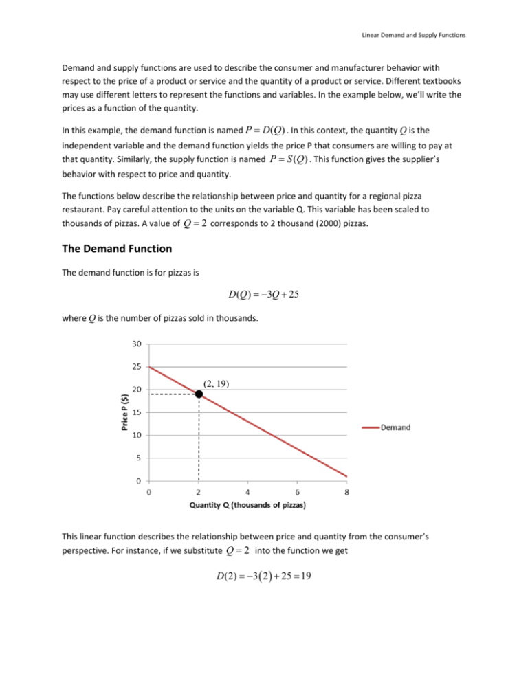
Linear Demand and Supply Functions Demand and supply functions are used to describe the consumer and manufacturer behavior with respect to the price of a product or service and the quantity of a product or service. Different textbooks may use different letters to represent the functions and variables. In the example below, we’ll write the prices as a function of the quantity. In this example, the demand function is named P  D(Q) . In this context, the quantity Q is the independent variable and the demand function yields the price P that consumers are willing to pay at that quantity. Similarly, the supply function is named P  S (Q ) . This function gives the supplier’s behavior with respect to price and quantity. The functions below describe the relationship between price and quantity for a regional pizza restaurant. Pay careful attention to the units on the variable Q. This variable has been scaled to thousands of pizzas. A value of Q  2 corresponds to 2 thousand (2000) pizzas. The Demand Function The demand function is for pizzas is D (Q )  3Q  25
where Q is the number of pizzas sold in thousands. (2, 19)
This linear function describes the relationship between price and quantity from the consumer’s perspective. For instance, if we substitute Q  2 into the function we get D (2)  3  2   25  19 Linear Demand and Supply Functions This means that at a price of $19, consumers demand 2 thousand pizzas. In addition to finding the price corresponding to a quantity, we can reverse the process. To find the quantity of pizzas corresponding to a price of $13, set the demand function equal to 13 and solve for Q: 13  3Q  25
12  3Q
4Q
Subtract 25 from both sides
Divide both sides by ‐3
This means that at a price of $13 per pizza, a quantity of 4 thousand pizzas will be demanded by consumers. The graph also makes sense. On the left side of the graph, prices are high and the quantity sold is low. In other words, consumers are reluctant to purchase pizzas when the price is high. On the right side of the graph, the quantity is high and the price is low. This means that demand is higher when the price is lower. This type of relationship, a decreasing linear function, is often an excellent model for reality. High quantity demanded at a low price
Low quantity demanded
at high price The Supply Function A supply function models the relationship between price and quantity with respect to the manufacturer. Suppose the supply function for the pizza restaurant chain is S (Q)  2Q . The graph below shows this supply function. Linear Demand and Supply Functions Unlike the demand curve which was decreasing, this curve increases. Let’s look at parts of this curve closer to insure that it makes sense. Low quantity supplied at a low price
High quantity supplied at high price
Points on the left side of the graph show a low quantity and a low price. This means that at a low price, the pizza restaurant will be willing to supply a low quantity of pizzas per week. Points on the right side of the graph show a high price and a high quantity. This means that at a high price, the pizza restaurant will be willing to supply a high quantity of pizzas per week. This behavior is exactly what you would expect from a supplier. But it points to an interesting irony. The pizza restaurant wants to supply higher numbers of pizzas per week when the price is high. But when the price is high, the number of pizzas sold is low. We can also look at it differently by noting that when the price is low, the pizza restaurant doesn’t want to sell many pizzas but the consumers want to buy more. Is there a quantity and price which will satisfy the pizza restaurant and the consumer? Linear Demand and Supply Functions The Equilibrium Point To satisfy both the consumer and the manufacturer, we need to find a price and quantity on each curve where the price and quantity are exactly the same. At this price, the quantity demanded by consumers is the same as the quantity supplied by the manufacturer. This point is called the equilibrium point. The quantity at the equilibrium point is called the equilibrium quantity. The price at the equilibrium point is called the equilibrium price. It is easy to find this point on a graph. We simply need to find the point of intersection of the demand function D (Q ) and the supply curve S (Q ) . At this point, the value of P and Q are the same on both curves. From the graph above, we can see that the equilibrium point is at approximately (5, 10). This is an estimate based on the scaling on the graph. To find the point of intersection exactly, we need to find where the demand and supply curves are equal algebraically. How To Find the Equilibrium Point Algebraically The point of intersection of two graphs is found by setting the function’s formulas equal and solving for the variable. In the case of the supply and demand functions, we set S (Q)  D(Q) and solve for Q. When we set the supply and demand functions equal, we get 2Q  3Q  25 Linear Demand and Supply Functions Add 3Q to both sides to yield 5Q  25 Divide both sides by 5 and we get an equilibrium quantity of Q  5 . To get the equilibrium price, we need to put this quantity into either the supply function or the demand function: S (5)  2(5)  10
D (5)  3(5)  25  10
This means that at a price of $10 per pizza, the quantity demanded by consumers is 5000 pizzas and the quantity the pizza chain is willing to supply is 5000 pizzas. How To Find the Equilibrium Point Graphically Earlier we estimated the point of intersection from a graph. You can also use a graphing calculator to fine tune that estimate. To start, graph both functions in an appropriate window. Then we’ll use the CALC menu to find the point of intersection. 1. Enter the supply and demand functions into the equation editor by pressing the o button. You’ll need to use the „ button to type x in place of Q. 2. Press p to adjust the graphing window to the values shown to the right. 3. To see the graph, press s. Since the point of intersection is visible, we can move onto the next step. If the point of intersection is not visible, readjust the window by pressing p. Linear Demand and Supply Functions 4. To find the point of intersection, press yr to access the CALC menu. Use † to move your cursor to 5: intersect and press Í. 5. To find the point of intersection, you need to help the calculator by indicating the first curve and the second curve. Do this by moving the crosshairs to the appropriate curve with } or † and pressing Í to select the curve. 6. Now move the crosshairs with the | or ~ buttons near the point of intersection to supply the calculator with a starting guess. 7. Press Í to find the point of intersection. 8. The approximate point of intersection is displayed on the screen. Remember that this is an estimate. In this case, the estimate matches the exact answer we found algebraically.