Preserving Sharp Edges in Geometry Images
Mathieu Gauthier∗
Pierre Poulin
LIGUM, Dép. d’informatique et de recherche opérationnelle
Université de Montréal
A BSTRACT
A geometry image offers a simple and compact way of encoding the
geometry of a surface and its implicit connectivity in an image-like
data structure. It has been shown to be useful in multiple applications because of its suitability for efficient hardware rendering,
level of detail, filtering, etc. Most existing algorithms generate geometry images by parameterizing the surface onto a domain, and
by performing a regular resampling in this domain. Unfortunately,
this regular resampling fails to capture sharp features present on
the surface. In this paper, we propose to slightly alter the grid to
align sample positions with corners and sharp edges in the geometric model. While doing so, our goal is to maintain the resulting geometry images simple to interpret, while producing higher quality
reconstructions. We demonstrate an implementation in the planar
domain and show results on a range of common geometrical models.
Index Terms:
Representations—
1
I.3.5 [Computer Graphics]:
Surface
I NTRODUCTION
A geometry image [7] maps geometry into parametric space, from
which a regular mesh can be extracted. This space provides an implicit representation of the connectivity between vertices. However
regular sampling in this space without respecting sharp features in
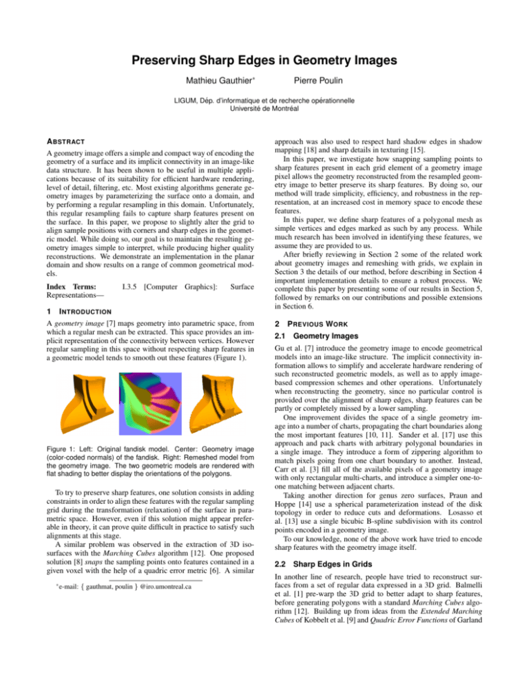
a geometric model tends to smooth out these features (Figure 1).
Figure 1: Left: Original fandisk model. Center: Geometry image
(color-coded normals) of the fandisk. Right: Remeshed model from
the geometry image. The two geometric models are rendered with
flat shading to better display the orientations of the polygons.
To try to preserve sharp features, one solution consists in adding
constraints in order to align these features with the regular sampling
grid during the transformation (relaxation) of the surface in parametric space. However, even if this solution might appear preferable in theory, it can prove quite difficult in practice to satisfy such
alignments at this stage.
A similar problem was observed in the extraction of 3D isosurfaces with the Marching Cubes algorithm [12]. One proposed
solution [8] snaps the sampling points onto features contained in a
given voxel with the help of a quadric error metric [6]. A similar
∗ e-mail:
{ gauthmat, poulin } @iro.umontreal.ca
approach was also used to respect hard shadow edges in shadow
mapping [18] and sharp details in texturing [15].
In this paper, we investigate how snapping sampling points to
sharp features present in each grid element of a geometry image
pixel allows the geometry reconstructed from the resampled geometry image to better preserve its sharp features. By doing so, our
method will trade simplicity, efficiency, and robustness in the representation, at an increased cost in memory space to encode these
features.
In this paper, we define sharp features of a polygonal mesh as
simple vertices and edges marked as such by any process. While
much research has been involved in identifying these features, we
assume they are provided to us.
After briefly reviewing in Section 2 some of the related work
about geometry images and remeshing with grids, we explain in
Section 3 the details of our method, before describing in Section 4
important implementation details to ensure a robust process. We
complete this paper by presenting some of our results in Section 5,
followed by remarks on our contributions and possible extensions
in Section 6.
2
2.1
P REVIOUS W ORK
Geometry Images
Gu et al. [7] introduce the geometry image to encode geometrical
models into an image-like structure. The implicit connectivity information allows to simplify and accelerate hardware rendering of
such reconstructed geometric models, as well as to apply imagebased compression schemes and other operations. Unfortunately
when reconstructing the geometry, since no particular control is
provided over the alignment of sharp edges, sharp features can be
partly or completely missed by a lower sampling.
One improvement divides the space of a single geometry image into a number of charts, propagating the chart boundaries along
the most important features [10, 11]. Sander et al. [17] use this
approach and pack charts with arbitrary polygonal boundaries in
a single image. They introduce a form of zippering algorithm to
match pixels going from one chart boundary to another. Instead,
Carr et al. [3] fill all of the available pixels of a geometry image
with only rectangular multi-charts, and introduce a simpler one-toone matching between adjacent charts.
Taking another direction for genus zero surfaces, Praun and
Hoppe [14] use a spherical parameterization instead of the disk
topology in order to reduce cuts and deformations. Losasso et
al. [13] use a single bicubic B-spline subdivision with its control
points encoded in a geometry image.
To our knowledge, none of the above work have tried to encode
sharp features with the geometry image itself.
2.2
Sharp Edges in Grids
In another line of research, people have tried to reconstruct surfaces from a set of regular data expressed in a 3D grid. Balmelli
et al. [1] pre-warp the 3D grid to better adapt to sharp features,
before generating polygons with a standard Marching Cubes algorithm [12]. Building up from ideas from the Extended Marching
Cubes of Kobbelt et al. [9] and Quadric Error Functions of Garland
and Heckbert [6], Ju et al. [8] introduce the concept of dual contouring to Hermite data over an octree of voxels. Their structure allows
to better reconstruct sharp features contained in a voxel. Wyvill and
van Overveld [20] propose an iterative refinement within a voxel to
reconstruct sharp junctions between CSG surfaces.
A number of applications of this concept in the 2D image space
have also been proposed. Sen et al. [18] store a number of line
segments due to shadow silhouettes in each pixel of a shadow map,
allowing to reconstruct sharp shadows cast within the shadow map
pixel. This concept is also used in a number of other applications,
including texturing [15].
However none of these works have studied the application of
their techniques to sharp edges in geometry images. This is the
main purpose of this paper.
3 P RESERVING S HARP F EATURES
We describe our algorithm as a series of modifications that need
to be applied to the traditional planar geometry image technique,
as introduced by Gu et al. [7]. While the same algorithm could
be implemented in other well-known geometry image generation
techniques, we will restrict ourselves to the traditional technique
for the sake of simplicity and generality.
Our input geometric model is assumed to be an orientable 2manifold polygonal surface that may contain holes and/or boundary components. We also assume that a mesh-cutting algorithm is
available to make the surface homeomorphic to a disk, as well as
an algorithm giving a parameterization inside the unit square that
respects the relative lengths of cut paths, thus allowing a seamless
reconstruction.
3.1 Grid Alignment to Sharp Features
We define a sharp edge as an edge of a geometric model where the
local edge dihedral angle of the two adjacent faces is larger than
a given threshold. Instead of a fixed threshold, smoothing group
information could also be used to identify sharp edges. We call a
corner a vertex of the geometric model adjacent to more than two
sharp edges and a sharp segment a series of sharp edges linking
two corners or looping back on itself. After loading, cutting, and
parameterizing our input geometric model, we extract the list of
sharp edges and sharp corners, and assign a unique identifier to each
sharp segment. Figure 2 shows an example with a simple model.
Figure 2: Sharp edges of a square torus in 3D and in its parametric
space. This example has 8 corners, 14 sharp segments, and many
sharp edges.
Our sampling domain is composed of a set of points that sample
the parameterization and generate a corresponding geometry image.
The data of one sample point is stored in one pixel in the geometry
image. For our purpose, the sampling domain is a regular grid in
the unit square. We explicitly instantiate it as a quad mesh at the
resolution set by the user, where each vertex represents a sample
point.
Superimposing the sampling domain grid over the surface parameterization can lead to the following observations. In parametric space, a sharp segment will be incorrectly sampled (hence incorrectly reconstructed) every time it crosses an edge between two
sample points. Ideally, all sharp segments should only cross the
grid at the exact location of a sample point. In the same way, every corner must also lie at a sample point. Figure 3 illustrates these
observations.
Figure 3: Top Left: In parametric space, a sharp edge (in red) will
be improperly sampled every time it crosses one of the domain grid
lines (in gray). Top Right: The poor reconstruction results from this
surface sampling. Bottom Left: Aligning the samples with the sharp
edge (in this example, by simply sliding them to the left or the right)
eliminates all crossings. Bottom Right: The reconstruction properly
captures these sharp features. Note that this example does not follow
the steps of our algorithm, but is merely an illustration of the sampling
problem.
To locally deform the sampling grid, as a first step, we locate the
domain sample closest to each corner vertex. We move each domain
sample to the position of the corresponding corner vertex, and store
the index of the corner vertex (from the mesh data structure) inside
the displaced domain sample for future reference. These samples
will not be allowed to move again. If the same domain sample is the
closest to more than one corner vertex, it will be displaced only to
the closest one, and the information from other nearby corner vertices will be neglected. Increasing the sampling domain resolution
would reduce some of these cases.
We process sharp edges in two passes. We first locate all intersections between sharp edges and grid edges. Note that grid edges
might have been displaced by the pass on corners. For each edgeedge intersection, we look at the two domain samples at each end
of the intersected grid edge. We select the sample between the two
that is closest to the intersection point, and check if this intersection is closer to the one found so far for this sample. Samples on
the boundaries of the parameterization are only allowed to move
along one axis, and the four corners are not allowed to move at all.
At the end of this pass, we assign the new computed positions of
the domain samples. We also mark the displaced samples so that
they cannot move again.
The second pass proceeds very similarly, and is needed when
multiple intersections occur in the vicinity of a domain sample. It
gives the algorithm a little more freedom to further improve on the
sampling quality. The only difference from the first pass is that we
allow to select the second-closest sample from an intersection in
cases where the closest sample has already been marked and moved
in the first pass.
Whenever we move a domain sample on a sharp edge, we associate the index of the mesh edge to the sample. We will later use
this information to sample surface normals.
Figure 4: A simple illustration of the steps of our algorithm using a model with 1 sharp corner and 4 sharp edges. The (x, y) coordinates are
defined inside the unit square and its parameterization is simply a projection on the xy-plane. Leftmost: The input model, the reconstruction
without grid alignment, and with our algorithm. From left to right: Unmodified 9 × 9 grid, corner snapping, first pass of edge snapping, second
pass.
3.2 Sampling
At this stage, the sampling grid is aligned to the corners and sharp
edges of the surface. The sampling of the parameterization can be
performed as with traditional geometry images, i.e., the grid sample positions sample directly the polygons in parametric space. uv
coordinates and normals form however two notable exceptions.
With a traditional geometry image sampled using a regular grid,
the uv coordinates simply coincide with the pixel’s relative position
on the grid. Since the sampling grid is now locally deformed, the
uv coordinates must be stored in an additional image or channel.
In order to be able to reconstruct the surface with its sharp features, we also have to store more than one surface normal for a given
sample point. For example, a sample point lying on a sharp edge
requires two different surface normals, while a corner may require
three or more surface normals. Our worst case scenario requires
up to 8 surface normals for a single sample point, and is illustrated
in Figure 5. This maximum of 8 normals comes from the number
of triangles that are generated during remeshing by a group of four
quads around a sample point.
Our goal is to store the surface normals in such a way that we
will be able to recreate the appropriate number of duplicate vertices
to represent the sampled sharp features.
We divide the neighborhood around each sample point into 8
logical octants, each one covering a triangle issued of the 4 neighboring quads (reconstructed from the 8 neighboring sample points)
originating from the vertex in the sampling domain. For each sample point, we store one surface normal per octant using the indexing
n1 , ..., n8 of Figure 5. This allows to associate different surface normals to different directions around the sample point.
We process the sample points of the grid one by one. If the current sample point has not been aligned to a sharp corner or a sharp
edge, we locate the triangle overlapping the sample point in parametric space. If this triangle does not share an edge or a vertex with
a sharp feature, we perform a standard barycentric interpolation of
the three normals for this triangle. Otherwise, we use the normal
of the triangle itself. We copy the resulting normal (interpolated
or from the triangle) to the 8 normals associated with the current
sample.
The assignment of normals to corners and sharp edges are described next, and illustrated in Figure 6.
n8
n1
n7
n2
n2
n2
n3
n8
n7
n4
v n6
n5
e
n6 n3
n3
n4
n5
n7
f1
v
n1
n8
n1
n4
f2
n6
n5
Figure 5: Sharp edges meeting at a sharp corner, with the maximum
allowed associated surface normals.
Figure 6: Left: Following each sharp edge originating from v identifies
three groups of octants (n8 , n1 , ..., n3 ), (n4 , n5 ), and (n6 , n7 ). Each
group receives the angle-weighted normal from the faces between a
pair of sharp edges. Right: The sharp edge e (in orange) is shared
by the two adjacent faces f1 and f2 (in gray). The normal of f1 is
copied in the octants (n1 , n2 , n8 ), while the normal of f2 covers the
remaining octants (n3 , ..., n7 ).
Several encoding schemes could be used to reduce the space required to store these normals. Each normal can first be encoded on
less bits. Moreover, since many samples will only need one normal,
and very few will need up to 8 normals, specialized data structures
can be adapted. Nevertheless, for simplicity sake, we decided to
store 8 normals per vertex, introducing redundancy where less than
8 normals are actually needed. The scheme has the advantage of
requiring a fixed size and is very much in line with the geometry
image philosophy. This also allows for a very simple remeshing
algorithm that will be described in Section 3.3.
If the sample point has been snapped to sharp corner v, the procedure is relatively simple. For each sharp edge originating at v, we
follow the sharp segment to identify the neighbor grid sample of
the 1-ring of v it reaches. In the general case, there are 8 neighbor
grid samples; there are less on the boundaries on the grid. Knowing which sharp edge leads to which neighbor grid sample, we iterate over the triangles around vertex v in counterclockwise order
and compute the angle-weighted normal between each pair of sharp
edges. The resulting normal is then copied to the corresponding octants.
When the sample point has been snapped to sharp edge e, it receives two normals, one from each face, f1 and f2 , adjacent to e.
The challenge is to assign the appropriate normal to the corresponding octants. We proceed very similarly to the vertex case. For each
half-edge of e, we follow the sharp segment in a forward manner
to verify which one of the neighbor grid samples it is connected to.
Knowing the samples reached in each direction and the face ( f1 or
f2 associated to each half-edge, we copy the normal of f1 and f2 in
the corresponding octants.
In poorly sampled regions, it can happen that two neighbor grid
samples cannot be reached. In this case, we simply copy the
weighted average normal at the vertex to all its surrounding octants. When the sampling grid is much finer than the original mesh
triangles, it is possible that more than one neighbor grid sample is
snapped to the same sharp edge. In this case, we always take the
closest one from v on the outgoing edge segment. This is illustrated
in Figure 7.
n2
n2
n3
n7
f2
f1
n6
n4
n5
n6
n1 n8
n4 n5
n1 n8
n4 n5
n7
n6
n2
n3
n7
n6
n2
n3
n3/ n4
n1 n8
n4 n5
n1 n8
n4 n5
n7
n6
n7
n6
n5/ n6
n3
n4
n5
Figure 7: When the grid resolution is much finer than the original
mesh triangles, multiple samples can be assigned to the same sharp
edge. In each direction, we only consider the closest sample (in the
appropriate direction) from the current one. Here, octants (n1 , ..., n4 )
receive the normal of f1 and octants (n5 , ..., n8 ) receive the normal of
f2 .
Sampling an edge or a corner located on the boundary of the parameterization requires more careful bookkeeping. This is due to
the fact that cutting a surface into a disk will necessarily create duplicate (or mate) vertices on the boundary of the parameterization,
and therefore the 1-ring of a domain sample may spread in two or
more regions of the parameterization. Since the 1-ring may include
more than 8 vertices, the notion of octant does not translate very
well in these cases. For this reason, we first process each grid sample ignoring mate vertices. As a post-process, we then locate the
sharp segments jumping from one area of the grid to another, and
average the corresponding octant normals on each side of the sharp
segment.
3.3
n2
n3
n8
n1
n3
used to determine the triangulation, such as trying to minimize edge
lengths or aspect ratios in 3D.
The four vertices composing each quad have up to 8 possible
normals. We render them as two triangles and determine which
normal to use in the temporary array, with the indexing scheme
illustrated in Figure 8. This automatically recreates the sharp edges
where they are needed.
Remeshing
Reconstructing the surface from the position geometry image and
the normal geometry image is quite simple. For each pixel in the
position geometry image, we create as many vertices as there are
different normals in the normal geometry image. We keep those
vertices in a temporary array of 8 elements corresponding to each
octant of the sample. In the simplest case where no sharp features are associated with this sample, the 8 elements will contain
the same and unique vertex.
When all the vertices are created, we create a quad for each group
of four adjacent pixels. There are two ways of triangulating a quad.
When a sharp feature crosses the quad diagonally, we align the diagonal of the quad with it, so that the sharp edge will be correctly
represented. The orientation of the triangulation is determined during surface sampling and requires one extra bit in the geometry image. When no sharp feature traverses the quad, any strategy can be
n7 / n8
n1
n2
n7
n8
n1/ n2
Figure 8: There are two possible ways of triangulating a quad when
reconstructing the surface. Top: The shaded quad and its 4 vertices
(image pixels), each having 8 normals in its octants. Bottom: Normals to use for each diagonal configuration. In some cases, there
are two choices of normals to use.
4 I MPLEMENTATION
We have implemented the complete method of Gu et al. [7] in C++,
and then added the modifications described in Section 3. All our
mesh operations use a half-edge data structure.
To cut the mesh into a disk before the parameterization, we found
that allowing the cut path to follow a sharp segment or to go through
a sharp corner constrains too much the freedom of the algorithm,
since the resulting boundary samples are only allowed to move
along one axis. Therefore in all the results presented in this paper,
we manually defined the cut paths and avoided these situations.
To parameterize the mesh in the unit square, we use the geometric stretch energy as a combination of the area and angle distortions,
as proposed by Friedel et al. [5],
(
∞
if area( fD ) ≤ 0
Estretch ( f ) =
area( fM )2
·
E
otherwise
Dirichlet
area( f )2
D
where triangle f corresponds to triangle fM in the original mesh,
and to triangle fD in the parameterization domain. This type of
formulation is not practical to be used inside a black box nonlinear solver because it does not vary smoothly, as it reaches infinity
whenever a triangle flips in the parameterization space. Instead,
we use a 2D version of the combined energy function suggested by
Friedel et al. [5], which is a simple linear combination of the angle
and area distortions.
Ecombined = a · EDirichlet + b · Earea .
Our best results were obtained with lower (but non-null) angle
preservation (a = 0.01) and high area preservation (b = 1.0).
We coded, differentiated, and converted this energy function using Maple, a general-purpose commercial computer algebra system. The first and second derivatives were then fed to the NLS
unconstrained nonlinear solver of TAO [2]. A detailed discussion
on unconstrained parameterization and of this procedure, including
sample code, can be found in the Ph.D. thesis of Friedel [4].
We build a progressive mesh sequence, similarly to the approach
of Sander et al. [16], to derive an initial parameterization. First the
mesh is decimated using a quadric error metric, but without removing vertices located on the boundary. Since the mesh is cut to be
made homeomorphic to a disk, the base mesh will simply consist
of the boundary, plus a single vertex. The boundary is parameterized around the unit square in a way similar to Gu et al. [7], and the
remaining vertex is positioned at the center.
Then, at each iteration, we double the number of vertices, positioning each new vertex at the barycenter of the kernel of its neighbors in parameterization space. Every time the number of vertices
has increased by a certain factor, we launch the optimization process. Because we perform splits in the progressive mesh sequence,
tiny (almost null-area) triangles may be created. We set a minimum face area (10−8 ) to keep the optimization process stable. The
resulting process is illustrated in Figure 9.
249
499
999
1999
3999
7999
15999
31999
Figure 11: Top: Original fandisk model and averaging the 8 normal
geometry images. Bottom: Reconstruction at resolution 129 × 129
and reconstruction at 33 × 33 with superimposed wireframe mesh.
Our third example results from the union of a cube and a cylinder, and the subtraction of two cylinders on their respective cube
faces. Once again, the resulting geometrical model contains a combination of sharp edges and corners, and sharper edges resulting
from the intersection of the cylinders within the cube.
53056
Figure 9: Hierarchical parameterization of a hand model.
5
R ESULTS
Our first example (Figure 10) is obtained by subtracting a cylinder
from a cube. It has the topology of a torus, with 8 corners and
14 sharp segments. From left to right, we decrease the resolution
of the sampling grid to illustrate how the vertices are redistributed
over the geometrical model.
Figure 10: Top: Reconstruction of the square torus using a regular
sampling with grid resolutions of 65×65, 33×33, and 17×17. Bottom:
Our method using the same grid resolutions.
Our second example is the fandisk (Figure 11), commonly used
in several remeshing papers. This genus-0 surface contains a combination of sharp edges and corners, rounded corners, and progressively sharper edges. After applying our algorithm, vertices on
sharp edges were duplicated, creating a model from which continuous faces can be easily moved without affecting the other faces.
Figure 12: Top: Original pipe-hole model without and with wireframe.
Middle: Reconstruction at resolution 257 × 257 without and with wireframe. Bottom: Position geometry image and average of the 8 normal
geometry images.
6
C ONCLUSION
AND
F UTURE W ORK
A geometry image has proven to be an interesting structure to efficiently represent surfaces; a number of applications [19] have
therefore been introduced, exploiting this simplicity. In this paper, we presented a simple and efficient solution to retain in the
reconstructed surface the sharp edges and their respective normals.
Our algorithm should apply fairly straight-forwardly to most other
techniques based on geometry images, whether on spherical parameterizations, multi-charts, etc.
Because sharp features introduce the need to represent a number
of normals, our algorithm increased significantly the memory required to store them (actually a factor of 8 compared to the position
geometry image). While we did not try to compress these normals,
it should not be a difficult task, and should be studied in a future
implementation.
Another direction for improvements would refit our deformed
grid into a relaxation stage of the parameterization, thus resulting
hopefully in a regular grid, and avoiding the need for a uv coordinate image.
Finally, so far, we have only applied a greedy algorithm to snap
the closest grid point to a sharp edge or corner. We would like to
extend our transformation to obtain a more optimal and smoother
solution.
ACKNOWLEDGEMENTS
The authors thank Mohamed Yengui for discussions on sharp features, and constructive comments from anonymous reviewers. This
work was supported in parts by grants from NSERC.
R EFERENCES
[1] L. Balmelli, C. J. Morris, G. Taubin, and F. Bernardini. Volume warping for adaptive isosurface extraction. In VIS ’02: Proc. conference
on Visualization ’02, pages 467–474, 2002.
[2] S. Benson, L. C. McInnes, J. Moré, T. Munson, and J. Sarich. TAO
user manual (revision 1.9). Technical Report ANL/MCS-TM-242,
Mathematics and Computer Science Division, Argonne National Laboratory, 2007. http://www.mcs.anl.gov/tao.
[3] N. A. Carr, J. Hoberock, K. Crane, and J. C. Hart. Rectangular multichart geometry images. In SGP ’06: Proc. Eurographics symposium
on Geometry Processing, pages 181–190, 2006.
[4] I. Friedel. Approximation of Surfaces by Normal Meshes. PhD thesis,
California Institute of Technology, 2005.
[5] I. Friedel, P. Schröder, and M. Desbrun. Unconstrained spherical parameterization. In ACM SIGGRAPH 2005 Sketches, page 134, 2005.
[6] M. Garland and P. S. Heckbert. Surface simplification using quadric
error metrics. In SIGGRAPH ’97, pages 209–216, 1997.
[7] X. Gu, S. J. Gortler, and H. Hoppe. Geometry images. ACM Trans.
Graph., 21(3):355–361, 2002.
[8] T. Ju, F. Losasso, S. Schaefer, and J. Warren. Dual contouring of
Hermite data. ACM Trans. Graph., 21(3):339–346, 2002.
[9] L. P. Kobbelt, M. Botsch, U. Schwanecke, and H.-P. Seidel. Feature
sensitive surface extraction from volume data. In SIGGRAPH ’01,
pages 57–66, 2001.
[10] A. W. F. Lee, W. Sweldens, P. Schröder, L. Cowsar, and D. Dobkin.
Maps: multiresolution adaptive parameterization of surfaces. In SIGGRAPH ’98, pages 95–104, 1998.
[11] B. Lévy, S. Petitjean, N. Ray, and J. Maillot. Least squares conformal
maps for automatic texture atlas generation. In SIGGRAPH ’02, pages
362–371, 2002.
[12] W. E. Lorensen and H. E. Cline. Marching cubes: A high resolution 3D surface construction algorithm. SIGGRAPH Comput. Graph.,
21(4):163–169, 1987.
[13] F. Losasso, H. Hoppe, S. Schaefer, and J. Warren. Smooth geometry images. In Proc. Eurographics/ACM SIGGRAPH symposium on
Geometry Processing, pages 138–145, 2003.
[14] E. Praun and H. Hoppe. Spherical parametrization and remeshing.
ACM Trans. Graph., 22(3):340–349, 2003.
[15] G. Ramanarayanan, K. Bala, and B. Walter. Feature-based textures. In
Proc. Eurographics Symposium on Rendering, pages 265–274, 2004.
[16] P. V. Sander, J. Snyder, S. J. Gortler, and H. Hoppe. Texture mapping
progressive meshes. In SIGGRAPH ’01, pages 409–416, 2001.
[17] P. V. Sander, Z. J. Wood, S. J. Gortler, J. Snyder, and H. Hoppe. Multichart geometry images. In Proc. Eurographics/ACM SIGGRAPH symposium on Geometry Processing, pages 146–155, 2003.
[18] P. Sen, M. Cammarono, and P. Hanrahan. Shadow silhouette maps.
ACM Trans. Graph., 22(3):521–526, 2003.
[19] A. Sheffer, E. Praun, and K. Rose. Mesh parameterization methods
and their applications. Foundations and Trends in Computer Graphics
and Vision, 2(2):105–171, 2006.
[20] B. Wyvill and K. van Overveld. Polygonization of implicit surfaces with constructive solid geometry. Journal of Shape Modelling,
2(4):257–273, 1996.