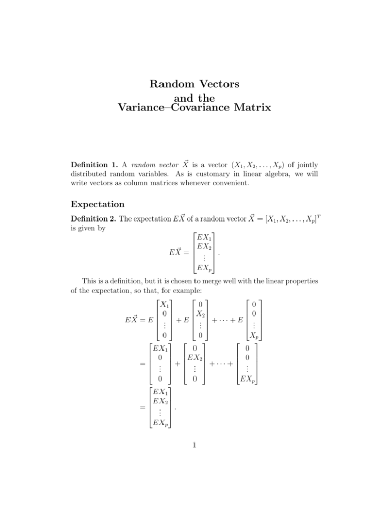
Random Vectors
and the
Variance–Covariance Matrix
~ is a vector (X1 , X2 , . . . , Xp ) of jointly
Definition 1. A random vector X
distributed random variables. As is customary in linear algebra, we will
write vectors as column matrices whenever convenient.
Expectation
~ of a random vector X
~ = [X1 , X2 , . . . , Xp ]T
Definition 2. The expectation E X
is given by


EX1
EX2 


~
E X =  ..  .
 . 
EXp
This is a definition, but it is chosen to merge well with the linear properties
of the expectation, so that, for example:
 
 
 
X1
0
0
0
X2 
0
 
 

~ =E
EX
 ..  + E  ..  + · · · + E  .. 
 . 
 . 
 . 
0
0
Xp

 



EX1
0
0
 0  EX2 
 0 



 

=  ..  +  ..  + · · · +  .. 
 .   . 
 . 
EXp
0
0


EX1
EX2 


=  ..  .
 . 
EXp
1
The linearity properties of the expectation can be expressed compactly by
stating that for any k × p-matrix A and any 1 × j-matrix B,
~ = AE X
~
E(AX)
~
~
and E(XB)
= (E X)B.
The Variance–Covariance Matrix
Definition 3. The variance–covariance matrix (or simply the covariance
~ is given by:
matrix ) of a random vector X
h
i
T
~
~
~
~
~
Cov(X) = E (X − E X)(X − E X) .
Proposition 4.
~ = E[X
~X
~ T ] − E X(E
~ X)
~ T.
Cov(X)
Proposition 5.

Var(X1 )
Cov(X1 , X2 )
Cov(X2 , X1 )
Var(X2 )
~ =
Cov(X)

..
..

.
.
Cov(Xp , X1 ) Cov(Xp , X2 )

· · · Cov(X1 , Xp )
· · · Cov(X2 , Xp )

.
..
..

.
.
···
Var(Xp )
~ is a symmetric matrix, since Cov(X, Y ) = Cov(Y, X).
Thus, Cov(X)
Exercise 1. Prove Propositions 4 and 5.
Linear combinations of random variables
Consider random variables X1 , . . . , Xp . We want to find the expectation
and variance of a new random variable L(X1 , . . . , Xp ) obtained as a linear
combination of X1 , . . . , Xp ; that is,
L(X1 , . . . , Xp ) =
p
X
ai X i .
i=1
Using vector–matrix notation we can write this in a compact way:
~ = ~aT X,
~
L(X)
2
where ~aT = [a1 , . . . , ap ]. Then we get:
~ = E[~aT X]
~ = ~aT E X
~ ,
E[L(X)]
and
~ = E[~aT X
~X
~ T ~a] − E(~aT X)[E(~
~
~ T
Var[L(X)]
aT X)]
~X
~ T ]~a − ~aT E X(E
~ X)
~ T ~a
= ~aT E[X
T
T
T
~
~
~
~
= ~a E[X X ] − E X(E X) ~a
~ a
= ~aT Cov(X)~
~ and Cov(X),
~ we can easily find the expectation and
Thus, knowing E X
variance of any linear combination of X1 , . . . , Xp .
Corollary 6. If Σ is the covariance matrix of a random vector, then for any
constant vector ~a we have
~aT Σ~a ≥ 0.
That is, Σ satisfies the property of being a positive semi-definite matrix.
Proof. ~aT Σ~a is the variance of a random variable.
This suggests the question: Given a symmetric, positive semi-definite
matrix, is it the covariance matrix of some random vector? The answer is
yes.
~ with covariance matrix Σ. Then,
Exercise 2. Consider a random vector X
for any k dimensional constant vector ~c and any p × k-matrix A, the k~ has mean ~c + AT E X
~ and has covariance
dimensional random vector ~c + AT X
matrix
~ = AT ΣA.
Cov(~c + AT X)
Exercise 3. If X1 , X2 , . . . , Xp are i.i.d. (independent identically distributed),
then Cov([X1 , X2 , . . . , Xp ]T ) is the p×p identity matrix, multiplied by a nonnegative constant.
Theorem 7 (Classical result in Linear Algebra). If Σ is a symmetric, positive
semi-definite matrix, there exists a matrix Σ1/2 (not unique) such that
(Σ1/2 )T Σ1/2 = Σ.
Exercise 4. Given a symmetric, positive semi-definite matrix Σ, find a random vector with covariance matrix Σ.
3
The Multivariate Normal Distribution
~ has the multivariate normal distribution
A p-dimensional random vector X
if it has the density function
1 ~
−p/2
−1/2
T −1 ~
~
f (X) = (2π)
|Σ|
exp − (X − µ
~ ) Σ (X − µ
~) ,
2
where µ
~ is a constant vector of dimension p and Σ is a p × p positive semidefinite which is invertible (called, in this case, positive definite). Then,
~ =µ
~ = Σ.
EX
~ and Cov(X)
The standard multivariate normal distribution is obtained when µ
~ = 0
and Σ = Ip , the p × p identity matrix:
1
T
−p/2
~ X
~ .
~ = (2π)
f (X)
exp − X
2
This corresponds to the case where X1 , . . . , Xp are i.i.d. standard normal.
Exercise 5. Let X1 and X2 be random variables with standard deviation σ1
and σ2 , respectively, and with correlation ρ. Find the variance–covariance
matrix of the random vector [X1 , X2 ]T .
Exercise 6 (The bivariate normal distribution). Consider a 2-dimensional
~ distributed according to the multivariate normal distriburandom vector X
tion (in this case called, for obvious reasons, the bivariate normal distribution). Starting with the formula for the density in matrix notation, derive
~ depending only on µ1 , µ2 (the means of X1
the formula for the density of X
and X2 ), σ1 , σ2 (the standard deviations of X1 and X2 ), and the correlation
coefficient ρ, and write it out without using matrix notation.
~ = [X1 , X2 ]T ,
Exercise 7. Consider a bivariate normal random vector X
~ = [5, −4]T , the standard deviations are StDev(X1 ) = 2 and
where E X
StDev(X2 ) = 3, and the correlation coefficient of X1 and X2 is −4/5. Use
~
R (or any other software package) to generate 100 independent draws of X,
and plot them as points on the plane.
Hint: To find Σ1/2 , find the eigenvalue decomposition of Σ as:
Σ = P DP T ,
4
where D is diagonal. Construct D1/2 by taking the square root of each diagonal entry, and define
Σ1/2 = P D1/2 P T .
In R, you can find the eigenvalue decomposition of Σ using:
ed <- eigen(sigma)
D <- diag(ed$values)
P <- ed$vectors
5