Pattern recognition systems – Lab 9
Linear Classifiers
1. Objectives
In this lab session we will study some linear discriminant functions like the
perceptron, and we will apply the gradient descent procedure for computing the best
classification rules for a two-class classification problem.
2. Theoretical Background
The goal of classification is to group items that have similar feature values into
classes or groups. A linear classifier achieves this goal by making a classification
decision based on the value of the linear combination of the features.
Definition of a classifier
Let S be a set of samples {S1, S2,…, Sn} that belong to m different classes
{c1, c2, … , cm}. Each sample has associated d features x = {x1, x2,…, xd}.
A classifier is a mapping from the feature space to the class labels {c1, c2,…,cm}.
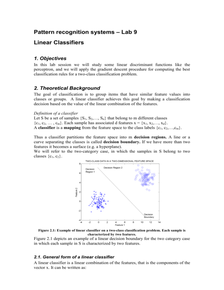
Thus a classifier partitions the feature space into m decision regions. A line or a
curve separating the classes is called decision boundary. If we have more than two
features it becomes a surface (e.g. a hyperplane).
We will refer to the two-category case, in which the samples in S belong to two
classes {c1, c2}.
Figure 2.1: Example of linear classifier on a two-class classification problem. Each sample is
characterized by two features.
Figure 2.1 depicts an example of a linear decision boundary for the two category case
in which each sample in S is characterized by two features.
2.1. General form of a linear classifier
A linear classifier is a linear combination of the features, that is the components of the
vector x. It can be written as:
d
g(x) = wT x + w0 = ∑ wi xi + w0
i =1
Where
• w is the weight vector
• w0 is the bias or the threshold weight
A two-category linear classifier (or binary classifier) implements the following
decision rule:
if g ( x) > 0 decide that sample x belongs to class c1

if g ( x) < 0 decide that sample x belongs to class c2
or
if w x > − w0 decide that sample x belongs to class c1

T
if w x < − w0 decide that sample x belongs to class c2
T
If g(x) = 0, x can ordinarily be assigned to either class.
2.2. Perceptron Learning
Consider the problem of learning a binary classification problem with a linear
classifier. Assume we have a dataset X={x(1, x(2,… , x(n} containing examples from
the two classes. Each sample x(i in the dataset is characterized by a feature vector {x1,
x2, … , xd}.
A schematic view of the perceptron is given in the next figure.
x1
w1
x2
xd
w2
wd
w0
1
f=w1x1+w2x2+…+wdxd+w0
T(f)
Weighted Sum of the inputs
Threshold
function
{c1,c2}
Output = Class decision
For convenience, we will absorb the intercept w0 by augmenting the feature vector x
with in additional constant dimension:
[
wT x + w0 = w0
]
1 
wT   = aT y
 x
Our objective is to find a vector such that :
 > 0, x ∈ c1
g ( x) = aT y 
< 0, x ∈ c2
To simplify the derivation, we will “normalize” the training set by replacing all
examples from class c2 by their negative: y ← [− y ], ∀y ∈ c2 .
This allows us to ignore class labels and look for a weight vector such that
aT y > 0, ∀y
To find the weight vector satisfying the above equation we define an objective
function J(a). The perceptron criterion function is:
J p (a) =
∑ (−a
T
y)
y∈ΥM
Where:
• YM is the set of samples misclassified by a
• Note that Jp(a) is non-negative since aTy<0 for all misclassified samples.
To find the minimum of this function, we use the gradient descent. The gradient is
defined by:
∇ a J p (a) = ∑ (− y )
y∈ΥM
The gradient descent update rule is:
a (k + 1) = a (k ) + η
∑y
y∈YM ( k )
This is known as perceptron batch update rule. Notice that the weight vector may be
updated in an “on-line” fashion, after the presentation of each individual example:
a (k + 1) = a (k ) + ηy (i , where y (i is an example that has been misclassified by a(k)
Algorithm: Batch Perceptron
Begin
• Initialize a, η, criterion θ, k=0
• “normalize” the training set by replacing all examples from class c2 by
their negative: y ← [− y ], ∀y ∈ c2
• Do
o k = k+1
o a=a+η ∑y
y∈YM (k)
•
Until η
∑ y <θ
y∈YM (k)
•
End
Return a
2.2.1. Numerical example
Compute the perceptron on the following dataset:
X1 = [(1,6), (7,2), (8,9), (9,9)]
X2 = [(2,1), (2,2), (2,4), (7,1)]
Perceptron leaning algorithm:
• Assume η=0.1
• Assume a(0)=[0.1, 0.1, 0.1]
• Use an online update rule
• Normalize the dataset
1 1 6


2
1 7
1 8 9


1 9 9

Y=
 −1 −2 −1 


 −1 −2 −2 
 −1 −2 −4 


 −1 −7 −1 
• Iterate through all the examples and update a(k) on the ones that are
misclassified
1. Y(1) ⇒ [1 1 6]*[0.1 0.1 0.1]T>0 ⇒ no update
2. Y(2) ⇒ [1 7 2]*[0.1 0.1 0.1]T>0 ⇒ no update
3. …
4. …
5. Y(5) ⇒ [-1 -2 -1]*[0.1 0.1 0.1]T<0 ⇒ update a(1) = [0.1 0.1 0.1] +
η*[-1 -2 -1] = [0 -0.1 0]
6. Y(6) ⇒ [-1 -2 -2]*[0 -0.1 0]T>0 ⇒ no update
7. …
8. Y(1) ⇒ [1 1 6]*[0 -0.1 0]T<0 ⇒ update a(2) = [0 -0.1 0] +η*[1 1 6]
= [0.1 0 0.6]
9. Y(2) ⇒ [1 7 2]*[0.1 0 0.6]T>0 ⇒ no update
10. …
Stop when η ∑ y < θ
y∈YM (k)
•
In this example, the perceptron rule converges after 175 iterations to
a=[-3.5 0.3 0.7]
3. Two-class two feature perceptron classifier
In our lab session we will find a perceptron linear classifier that discriminates
between two sets of points. The points in class 1 are colored in red and the points in
class 2 are colored in blue.
The figure below describes the dataset.
Figure 3.1: Input points for the perceptron classifier.
Each point is described by the color (that denotes the class label) and the two
coordinates, say x1 and x2.
The weights vector will have the form a = [w0, w1, w2].
The vector y = [ 1 x1 x2 ].
The algorithm becomes:
Algorithm: Batch Perceptron for two classes, two features
Begin
• Initialize
o a = [0.1 0.1 0.1]
o η=1
o stop threshold θ=0.00001
o k=0
o stop_vector b=[0 0 0]
•
“normalize” the training set by replacing all examples from class c2 by
their negative: y ← [− y ], ∀y ∈ c2 , hence y=[–1 –x1 –x2]
•
Do
o b = [0 0 0]
o k = k+1
o a=a+η ∑y
y∈YM (k)
o
b=b+η
∑y
y∈YM (k)
•
Until b < θ
•
Return a
End
The result of the classification is:
Figure 3.2: Result for the perceptron training
4. Exercices
Given a set of points belonging to two classes (red and blue):
Apply the batch perceptron algorithm to find the linear classifier that divides them
into two groups.
Consider η=1, initialize a(0) = [0.1, 0.1, 0.1] and θ=0.0001.
The palette of the input images is modified, such that on position 1 we have the color
red and on position 2 we have the color blue.
5. References
[1] Richard O. Duda, Peter E. Hart, David G. Stork: Pattern Classification 2nd ed.