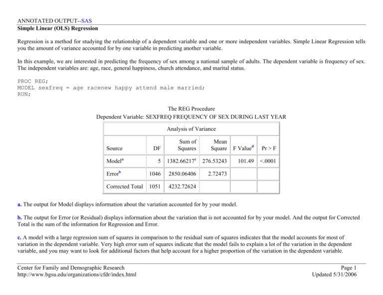
ANNOTATED OUTPUT--SAS
Simple Linear (OLS) Regression
Regression is a method for studying the relationship of a dependent variable and one or more independent variables. Simple Linear Regression tells
you the amount of variance accounted for by one variable in predicting another variable.
In this example, we are interested in predicting the frequency of sex among a national sample of adults. The dependent variable is frequency of sex.
The independent variables are: age, race, general happiness, church attendance, and marital status.
PROC REG;
MODEL sexfreq = age racenew happy attend male married;
RUN;
The REG Procedure
Dependent Variable: SEXFREQ FREQUENCY OF SEX DURING LAST YEAR
Analysis of Variance
Source
DF
Sum of
Squares
Mean
Square
F Valued
Pr > F
Modela
5
1382.66217c
276.53243
101.49
<.0001
Errorb
1046
2850.06406
2.72473
Corrected Total
1051
4232.72624
a. The output for Model displays information about the variation accounted for by your model.
b. The output for Error (or Residual) displays information about the variation that is not accounted for by your model. And the output for Corrected
Total is the sum of the information for Regression and Error.
c. A model with a large regression sum of squares in comparison to the residual sum of squares indicates that the model accounts for most of
variation in the dependent variable. Very high error sum of squares indicate that the model fails to explain a lot of the variation in the dependent
variable, and you may want to look for additional factors that help account for a higher proportion of the variation in the dependent variable.
Center for Family and Demographic Research
http://www.bgsu.edu/organizations/cfdr/index.html
Page 1
Updated 5/31/2006
ANNOTATED OUTPUT--SAS
d. If the significance value of the F statistic is small (smaller than say 0.05) then the independent variables do a good job explaining the variation in
the dependent variable. If the significance value of F is larger than say 0.05 then the independent variables do not explain the variation in the
dependent variable. For this example, the model does a good job explaining the variation in the dependent variable.
Root MSE
1.65067
R-Squaree
0.3267
Dependent Mean
2.75475
Adj R-Sq
0.3234
Coeff Var
59.92097
e. The “R Square” tells us how much of the variance of the dependent variable can be explained by the independent variable(s). In the case of Model
1, 20% of the variance in frequency of sex is explained by differences in age of respondent.
Parameter Estimates
DF
Parameter
Estimate
Standard
Error
t Valueg
Pr > |t|h
Intercept
1
8.29800
0.29663
27.97
<.0001
AGE
AGE OF RESPONDENT
1
-0.05550
0.00304
-18.26
<.0001
MARITAL
MARITAL STATUS
1
-1.37233
0.10713
-12.81
<.0001
RACENEW
NEW RACE RECODE
1
-0.21538
0.12527
-1.72
0.0859
ATTEND
HOW OFTEN R ATTENDS RELIGIOUS SERVICES
1
-0.06743
0.01962
-3.44
0.0006
HAPPY
GENERAL HAPPINESS
1
-0.26184
0.08464
-3.09
0.0020
Variable
Label
Interceptf
f. The “intercept” variable represents the Y-intercept, the height of the regression line when it crosses the Y axis. In this example, it is the predicted
value of “frequency of sex” when all other values are zero (0).
Center for Family and Demographic Research
http://www.bgsu.edu/organizations/cfdr/index.html
Page 2
Updated 5/31/2006
ANNOTATED OUTPUT--SAS
g. The t statistics can help you determine the relative importance of each variable in the model. As a guide regarding useful predictors, look for t
values well below -2 or above +2. For example, for “race” t = 1.72 and not significant.
h. The significance column indicates whether or not a variable is a significant predictor of the dependent variable. For example, the race variable is
not significant, while the other variables are significant.
Center for Family and Demographic Research
http://www.bgsu.edu/organizations/cfdr/index.html
Page 3
Updated 5/31/2006
ANNOTATED OUTPUT--SAS
Regression Equation
SEXFREQpredicted = 8.298 – .056*age – 1.372*marital - .215*race – .262*happy – .067*attend
For instance, if we plug in values in for the independent variables (age = 35 years; marital = currently married-1; race = white-1; happiness = very
happy-1; church attendance = never attends-0), we can predict a value for frequency of sex:
SEXFREQpredicted
= 8.298 – .056*35 – 1.372*1 - .215*1 – .262*1 – .067*0
= 4.489
As this variable is coded, a 35-year old, White, married person with high levels of happiness and who never attends church would be expected to
report their frequency of sex between values 4 (weekly) and 5 (2-3 times per week).
If we plug in 70 years, instead, we find that frequency of sex is predicted at 2.529, or approximately 1-2 times per month.
Model Interpretation
Intercept = The predicted value of “frequency of sex”, when all other variables are 0. In this example, a value of 8.298 is not interpretable, since the
valid responses for frequency of sex range from 0-6. Important to note, values of 0 for all variables is not interpretable either (i.e., age cannot equal
0).
Age = For every unit increase in age (in this case, year), frequency of sex will decrease by .056 units.
Marital Status = For every unit increase in marital status, frequency of sex will decrease by 1.372 units. Since marital status has only two categories,
we can conclude that currently married persons have more sex than currently unmarried persons.
Race = For every unit increase in race, frequency of sex will decrease by .215 units. Since race has only two categories, we can conclude that nonWhite persons have more sex than White persons.
Happiness = For every unit increase in happiness, frequency of sex will decrease by .262 units. Recall that happiness is coded such that higher scores
indicate less happiness. For this example, then, higher levels of happiness predict higher frequency of sex.
Church Attendance = For every unit increase in church attendance, frequency of sex decreases by .067 units.
Center for Family and Demographic Research
http://www.bgsu.edu/organizations/cfdr/index.html
Page 4
Updated 5/31/2006
ANNOTATED OUTPUT--SAS
Simple Linear Regression (with non-linear variable)
PROC REG;
MODEL sexfreq = age marital racenew happy church agesquar;
RUN;
It is known that some variables are often non-linear, or curvilinear. Such variables may be age or income. In this example, we include the original age
variable and an age squared variable.
Parameter Estimates
DF
Parameter
Estimate
Standard
Error
t Value
Pr > |t|
Intercept
1
7.46680
0.49979
14.94
<.0001
AGE
AGE OF RESPONDENT
1
-0.02050
0.01722
-1.19
0.2343
MARITAL
MARITAL STATUS
1
-1.31425
0.11060
-11.88
<.0001
RACENEW
NEW RACE RECODE
1
-0.21831
0.12508
-1.75
0.0812
HAPPY
GENERAL HAPPINESS
1
-0.27140
0.08464
-3.21
0.0014
ATTEND
HOW OFTEN R ATTENDS RELIGIOUS SERVICES
1
-0.06707
0.01959
-3.42
0.0006
1
-0.00035233
0.00017065
-2.06
0.0392
Variable
Label
Intercept
AGESQUARi
i. The age squared variable is significant, indicating that age is non-linear.
Center for Family and Demographic Research
http://www.bgsu.edu/organizations/cfdr/index.html
Page 5
Updated 5/31/2006
ANNOTATED OUTPUT--SAS
Simple Linear Regression (with interaction term)
In a linear model, the effect of each independent variable is always the same. However, it could be that the effect of one variable depends on another.
In this example, we might expect that the effect of marital status is dependent on gender. In the following example, we include an interaction term,
male*married.
To test for two-way interactions (often thought of as a relationship between an independent variable (IV) and dependent variable (DV), moderated by
a third variable), first run a regression analysis, including both independent variables (IV and moderator) and their interaction (product) term. It is
highly recommended that the independent variable and moderator are standardized before calculation of the product term, although this is not
essential.
For this example, two dummy variables were created, for ease of interpretation. Gender was coded such that 1=Male and 0=Female. Marital status
was coded such that 1=Currently married and 0=Not currently married. The interaction term is a cross-product of these two dummy variables.
Center for Family and Demographic Research
http://www.bgsu.edu/organizations/cfdr/index.html
Page 6
Updated 5/31/2006
ANNOTATED OUTPUT--SAS
Regression Model (without interactions)
PROC REG;
MODEL sexfreq = age racenew happy attend male married;
RUN;
Parameter Estimates
DF
Parameter
Estimate
Standard
Error
t Value
Pr > |t|
Variable
Label
Intercept
Intercept
B
7.93136
0.31097
25.51
<.0001
AGE
AGE OF RESPONDENT
1
-0.05477
0.00303
-18.09
<.0001
MARITAL
MARITAL STATUS
B
-1.31795
0.10748
-12.26
<.0001
RACENEW
NEW RACE RECODE
1
-0.23077
0.12458
-1.85
0.0643
HAPPY
GENERAL HAPPINESS
1
-0.24217
0.08430
-2.87
0.0042
ATTEND
HOW OFTEN R ATTENDS RELIGIOUS SERVICES
1
-0.05626
0.01974
-2.85
0.0045
MALE
Male
1
0.38525
0.10387
3.71
0.0002
MARRIED
Married
0
0
.
.
.
Center for Family and Demographic Research
http://www.bgsu.edu/organizations/cfdr/index.html
Page 7
Updated 5/31/2006
ANNOTATED OUTPUT--SAS
Regression Model (with interactions)
PROC REG;
MODEL sexfreq = age racenew happy attend male married interact;
RUN;
Parameter Estimates
DF
Parameter
Estimate
Standard
Error
t Value
Pr > |t|
Variable
Label
Intercept
Intercept
1
4.90172
0.24802
19.76
<.0001
AGE
AGE OF RESPONDENT
1
-0.05387
0.00306
-17.63
<.0001
RACENEW
NEW RACE RECODE
1
-0.22534
0.12409
-1.82
0.0697
HAPPY
GENERAL HAPPINESS
1
-0.23012
0.08389
-2.74
0.0062
MALE
Male
1
0.72980
0.13809
5.29
<.0001
MARRIED
Married
1
1.60935
0.14769
10.90
<.0001
INTERACT
Interact
1
-0.67733
0.20924
-3.24
0.0012
The product term should
be significant in the
regression equation in
order for the interaction to
be interpretable.
Regression Equation
SEXFREQpredicted = 4.902 -.054*age - .225*race -.230*happy + 1.609*married + (.730 - .677*married) * male
Interpretation
Main Effects
The married coefficient represents the main effect for females (the 0 category). The effect for females is then 1.61, or the “marital”
coefficient. The effect for males is 1.61 - .68, or .93.
Center for Family and Demographic Research
http://www.bgsu.edu/organizations/cfdr/index.html
Page 8
Updated 5/31/2006
ANNOTATED OUTPUT--SAS
The gender coefficient represents the main effect for unmarried persons (the 0 category). The effect for unmarried is then .73, or the “sex”
coefficient. The effect for married is .73 - .68, or .05.
Interaction Effects
For a simple interpretation of the interaction term, plug values into the regression equation above.
Married Men =
Married Women =
Unmarried Men =
Unmarried Women =
SEXFREQpredicted = 4.902 -.054*age - .225*race -.230*happy + 1.609*1 + (.730 - .677*1) * 1
SEXFREQpredicted = 4.902 -.054*age - .225*race -.230*happy + 1.609*1 + (.730 - .677*1) * 0
SEXFREQpredicted = 4.902 -.054*age - .225*race -.230*happy + 1.609*0 + (.730 - .677*0) * 1
SEXFREQpredicted = 4.902 -.054*age - .225*race -.230*happy + 1.609*0 + (.730 - .677*0) * 0
= 4.219
= 4.166
= 2.610
= 2.557
In this example (age = 35 years; race = white-1; happiness = very happy-1; church attendance = never attends-0), we can see that (1) for both married
and unmarried persons, males are reporting higher frequency of sex than females, and (2) married persons report higher frequency of sex than
unmarried persons. The interaction tells us that the gender difference is greater for married persons than for unmarried persons.
Center for Family and Demographic Research
http://www.bgsu.edu/organizations/cfdr/index.html
Page 9
Updated 5/31/2006