Learning Plan Rewriting Rules
José Luis Ambite, Craig A. Knoblock & Steven Minton
Information Sciences Institute
University of Southern California
4676 Admiralty Way, Marina del Rey, CA 90292, USA
{ambite, knoblock, minton}@isi.edu
Abstract
Planning by Rewriting (PbR) is a new paradigm for efficient high-quality planning that exploits plan rewriting rules and efficient local search techniques to transform an easy-to-generate, but possibly suboptimal,
initial plan into a high-quality plan. Despite the advantages of PbR in terms of scalability, plan quality, and anytime behavior, PbR requires the user to
define a set of domain-specific plan rewriting rules
which can be difficult and time-consuming. This paper presents an approach to automatically learning the
plan rewriting rules based on comparing initial and optimal plans. We report results for several planning domains showing that the learned rules are competitive
with manually-specified ones, and in several cases the
learning algorithm discovered novel rewriting rules.
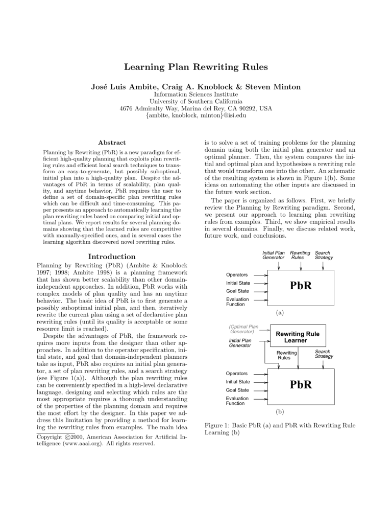
is to solve a set of training problems for the planning
domain using both the initial plan generator and an
optimal planner. Then, the system compares the initial and optimal plan and hypothesizes a rewriting rule
that would transform one into the other. An schematic
of the resulting system is shown in Figure 1(b). Some
ideas on automating the other inputs are discussed in
the future work section.
The paper is organized as follows. First, we briefly
review the Planning by Rewriting paradigm. Second,
we present our approach to learning plan rewriting
rules from examples. Third, we show empirical results
in several domains. Finally, we discuss related work,
future work, and conclusions.
Initial Plan
Generator
Introduction
Planning by Rewriting (PbR) (Ambite & Knoblock
1997; 1998; Ambite 1998) is a planning framework
that has shown better scalability than other domainindependent approaches. In addition, PbR works with
complex models of plan quality and has an anytime
behavior. The basic idea of PbR is to first generate a
possibly suboptimal initial plan, and then, iteratively
rewrite the current plan using a set of declarative plan
rewriting rules (until its quality is acceptable or some
resource limit is reached).
Despite the advantages of PbR, the framework requires more inputs from the designer than other approaches. In addition to the operator specification, initial state, and goal that domain-independent planners
take as input, PbR also requires an initial plan generator, a set of plan rewriting rules, and a search strategy
(see Figure 1(a)). Although the plan rewriting rules
can be conveniently specified in a high-level declarative
language, designing and selecting which rules are the
most appropriate requires a thorough understanding
of the properties of the planning domain and requires
the most effort by the designer. In this paper we address this limitation by providing a method for learning the rewriting rules from examples. The main idea
c
Copyright °2000,
American Association for Artificial Intelligence (www.aaai.org). All rights reserved.
Rewriting Search
Rules
Strategy
Operators
Initial State
PbR
Goal State
Evaluation
Function
(a)
(Optimal Plan
Generator)
Initial Plan
Generator
Rewriting Rule
Learner
Rewriting
Rules
Search
Strategy
Operators
Initial State
PbR
Goal State
Evaluation
Function
(b)
Figure 1: Basic PbR (a) and PbR with Rewriting Rule
Learning (b)
Review of Planning by Rewriting
Planning by Rewriting is a local search method (Aarts
& Lenstra 1997; Papadimitriou & Steiglitz 1982) for
domain-independent plan optimization. A brief summary of the main issues follows (see (Ambite 1998) for
a detailed description):
• Efficient generation of an initial solution plan. In
many domains obtaining a possibly suboptimal initial plan is easy. For example, in the Blocks World
it is straightforward to generate a solution in linear
time using the naive algorithm: put all blocks on the
table and build the desired towers from the bottom
up (like the plan in Figure 3(a)).
• Definition and application of the plan rewriting
rules. The user (or a learning algorithm) specifies
the appropriate rewriting rules for a domain in a simple declarative rule definition language. These rules
are matched against the current plan and generate
new transformed plans of possibly better quality.
• Plan quality measure. This is the plan cost function
of the application domain which is optimized during
the rewriting process.
• Searching of the space of rewritings. There are many
possible ways of searching the space of rewritten
plans, for example, gradient descent, simulated annealing, etc.
In Planning by Rewriting a plan is represented by
a graph, in the spirit of partial-order causal-link planners such as UCPOP (Penberthy & Weld 1992). The
nodes are domain actions. The edges specify a temporal ordering relation among nodes, imposed by causal
links and ordering constraints. The operator definition
language of PbR is the same as that of Sage (Knoblock
1995), which adds resources and run-time variables to
UCPOP. Figure 2 shows the specification of a simple
Blocks World planning domain. Two sample plans using this domain appear in Figure 3.
(define (operator stack)
:parameters (?X ?Y ?Z)
:precondition
(:and (on ?X ?Z) (clear ?X) (clear ?Y)
(:neq ?Y ?Z) (:neq ?X ?Z) (:neq ?X ?Y)
(:neq ?X Table) (:neq ?Y Table))
:effect (:and (on ?X ?Y) (:not (on ?X ?Z))
(clear ?Z) (:not (clear ?Y))))
(define (operator unstack)
:parameters (?X ?Y)
:precondition
(:and (on ?X ?Y) (clear ?X) (:neq ?X ?Y)
(:neq ?X Table) (:neq ?Y Table))
:effect (:and (on ?X Table) (:not (on ?X ?Y))
(clear ?Y)))
Figure 2: Planning Operators Specification
clear(B)
Causal Link
Ordering Constraint
Side Effect
on(A Table)
on(C A)
clear(A)
on(C Table)
on(C A)
clear(C)
on(D Table)
on(A Table)
clear(B)
3 STACK(A B Table)
4 UNSTACK(C A)
on(B Table)
on(A B)
clear(C)
on(B C)
2 STACK(B C Table)
clear(C)
on(C D)
0
1 STACK(C D Table)
GOAL
clear(D)
clear(B)
on(C Table)
clear(D)
A
on(B D)
B
on(B Table)
5 UNSTACK(B D)
on(B D)
clear(B)
C
B
A
D
C
D
clear(C)
Initial State
Goal State
(a) Initial Plan
on(A Table)
clear(B)
on(A Table)
3 STACK(A B Table)
clear(B)
clear(A)
on(D Table)
on(C A)
on(B Table)
on(A B)
clear(C)
on(B C)
2 STACK(B C Table)
clear(C)
on(C D)
6 STACK(C D A)
0
clear(B)
GOAL
clear(D)
on(C A)
clear(D)
Causal Link
Ordering Constraint
Side Effect
on(B D)
on(B Table)
5 UNSTACK(B D)
on(B D)
clear(B)
C
B
A
D
A
B
C
D
clear(C)
Initial State
Goal State
(b) Optimal Plan
Figure 3: PbR Plans
A plan rewriting rule specifies declaratively the replacement under certain conditions of a subplan by
another subplan. These rules are intended to improve
the quality of the plans. Plan rewriting rules arise from
algebraic properties of the operators in a planning domain. For example, a rule may state that two subplans
are equivalent for the purposes of achieving some goals,
but one of the subplans is preferred. Figure 4 shows
two rules for the Blocks World domain of Figure 2.
Intuitively, the avoid-move-twice rule says that it is
preferable to stack a block on top of another directly,
rather than first moving it to the table. Similarly, the
avoid-undo rule states that moving a block to the table and immediately putting it back to where it was
originally is useless, and thus if two such steps appear
in a plan, they can be removed. The application of
the avoid-move-twice rule to the plan in Figure 3(a)
produces the plan in Figure 3(b) (steps 4 and 1 are
replaced by step 6; ?b1 = C, ?b2 = A, ?b3 = D).
PbR has been successfully applied to several planning domains, including query planning in mediators
(Ambite & Knoblock 1998), but for clarity of exposition we will use examples from the Blocks World domain of Figure 2 throughout the paper. In the experimental results section we provide learning and performance results for the Blocks World, a process manufacturing domain, and a transportation logistics domain.
Learning Plan Rewriting Rules
In this section we describe our algorithms for proposing plan rewriting rules and for converging on a set of
useful rewriting rules.
(define-rule :name avoid-move-twice
:if (:operators ((?n1 (unstack ?b1 ?b2))
(?n2 (stack ?b1 ?b3 Table)))
:links (?n1 (on ?b1 Table) ?n2)
:constraints ((possibly-adjacent ?n1 ?n2)
(:neq ?b2 ?b3)))
:replace (:operators (?n1 ?n2))
:with (:operators (?n3 (stack ?b1 ?b3 ?b2))))
(define-rule :name avoid-undo
:if (:operators ((?n1 (unstack ?b1 ?b2))
(?n2 (stack ?b1 ?b2 Table)))
:constraints ((possibly-adjacent ?n1 ?n2))
:replace (:operators (?n1 ?n2))
:with nil))
Figure 4: Rewriting Rules (Blocks World)
Rule Generation
The main assumption of our learning algorithm is that
useful rewriting rules are of relatively small size (measured as the number of nodes and edges in the rule).
If a domain requires large rewriting rules, it is probably not a good candidate for a local search, iterative
repair algorithm such as PbR. Previous research also
lends support for biases that favor conciseness (Minton
& Underwood 1994). The rule generation algorithm
follows these steps:
1. Problem Generation. To start the process, our
algorithm needs a set of training problems for the planning domain. The choice of training problems determines the rules learned. Ideally, we would like problems drawn from the target problem distribution that
generate plans gradually increasing in size (i.e., number of plan steps) in order to learn the smallest rewriting rules first. Towards this end we have explored two
heuristics, based on a random problem generator, that
work well in practice. For some domains the size of
the plans can be controlled accurately by the number
of goals. Thus, our system generates sets of problems
increasing the number of goals up to a given goal size.
For each goal size the system generates a number of
random problems. We used this heuristic in our experiments. An alternative strategy is to generate a large
number of problems with different goal sizes, sort the
resulting plans by increasing size, and select the first
N to be the training set.
2. Initial Plan Generation. For each domain, we
define an initial plan generator. For example, the plan
in Figure 3(a) was generated by putting all blocks on
the table and building the desired towers from the bottom up. How to obtain in general such initial plan generators is beyond the scope of this paper, but see the
discussion in the future work section and in (Ambite
1998) for some approaches.
3. Optimal Plan Generation. Our algorithm
uses a general purpose planner performing a complete
search according to the given cost metric to find the
optimal plan. This is feasible only because the training
problems are small; otherwise, the search space of the
complete planner would explode. In our implementation we have used IPP (Koehler et al. 1997) and Sage
(Knoblock 1995) as the optimal planners. Figure 3(b)
shows the optimal plan for the problem in Figure 3(a).
4. Plan Comparison. Both the initial and optimal
plans are ground labeled graphs (see Figure 3). Our
algorithm performs graph differences between the initial and the optimal plans to identify nodes and edges
present in only one of the plans. Formally, an intersection graph Gi of two graphs G1 and G2 is a maximal subgraph isomorphism between G1 and G2 . If
in a graph there are nodes with identical labels, there
may be several intersection graphs. Given a graph intersection Gi , a graph difference G1 − G2 is the subgraph of G1 whose nodes and edges are not in Gi .1
In the example in Figure 3, the graph difference between the initial and the optimal plans, Gini − Gopt ,
is the graph formed by the nodes: unstack(C A)
and stack(C D Table); and the edges: (0 clear(C)
1), (0 clear(C) 4), (0 on(C A) 4), (1 on(C D)
Goal), (4 clear(A) 3), (4 on(C Table) 1), (5
clear(D) 1), and (1 2). Similarly, Gopt − Gini is
formed by the nodes: stack(C D A), and the edges:
(6 clear(A) 3), (5 clear(D) 6), (0 clear(C) 6),
(0 on(C A) 6), (6 on(C D) Goal), and (6 2).
5. Ground Rule Generation. After the plan comparison, the nodes and edges present only in the initial
plan form the basis for the antecedent of the rule, and
those present only in the optimal plan form the basis
for the consequent. In order to maximize the applicability of the rule, not all the differences in nodes and
edges of the respective graphs are included. Specifically, if there are nodes in the difference, only the edges
internal to those nodes are included in the rule. This
amounts to removing from consideration the edges
that link the nodes to the rest of the plan. In other
words, we are generating partially-specified rules.2 In
our example, the antecedent nodes are unstack(C A)
1
Our implementation performs a simple but efficient approximation to graph difference. It simply computes the
set difference on the set of labels of nodes (i.e., the ground
actions) and on the “labeled” edges (i.e., the causal or ordering links with each node identifier substituted by the
corresponding node action).
2
A partially-specified rule (Ambite 1998) states only the
most significant aspects of a transformation, as opposed to
the fully-specified rules typical of graph rewriting systems.
The PbR rewriting engine fills in the details and checks
for plan validity. If a rule is overly general, it may fail
to produce a rewriting for a plan that matches the rule’s
antecedent, but it would never produce an invalid plan.
(node 4) and stack(C D Table) (node 1). Therefore,
the only internal edge is (4 on(C Table) 1). This
edge is included in the rule antecedent and the other
edges are ignored. As the consequent is composed
of only one node, there are no internal edges. Rule
bw-1-ground in Figure 5 is the ground rule proposed
from the plans of Figure 3.
If there are only edge (ordering or causal link) differences between the antecedent and the consequent, a
rule including only edge specifications may be overly
general. To provide some context for the application
of the rule our algorithm includes in the antecedent
specification those nodes participating in the differing
edges (see rule sc-14 in Figure 9 for an example).
The algorithm for proposing ground rules described
in the preceding paragraphs is one point in a continuum from fully-specified rules towards more partiallyspecified rules. The main issue is that of context. In
the discussion section we expand on how context affects the usefulness of the rewriting rules.
6. Rule Generalization. Our algorithm generalizes the ground rule conservatively by replacing constants by variables, except when the schemas of the
operators logically imply a constant in some position of a predicate (similarly to EBL (Minton 1988)).
Rule bw-1-generalized in Figure 5 is the generalization of rule bw-1-ground which was learned from the
plans of Figure 3. The constant Table remains in the
bw-1-generalized rule as is it imposed by the effects
of unstack (see Figure 2).
(define-rule :name bw-1-ground
:if (:operators ((?n1 (unstack C A))
(?n2 (stack C D Table)))
:links (?n1 (on C Table) ?n2))
:replace (:operators (?n1 ?n2))
:with (:operators (?n3 (stack C D A))))
(define-rule :name bw-1-generalized
:if (:operators ((?n1 (unstack ?b1 ?b2))
(?n2 (stack ?b1 ?b3 Table)))
:links (?n1 (on ?b1 Table) ?n2))
:replace (:operators (?n1 ?n2))
:with (:operators (?n3 (stack ?b1 ?b3 ?b2))))
Figure 5: Ground vs. Generalized Rewriting Rules
Biasing towards Small Rules
There may be a large number of differences between
an initial and an optimal plan. These differences are
often better understood and explained as a sequence
of small rewritings than as the application of a large
monolithic rewriting. Therefore, in order to converge
to a set of small “primitive” rewriting rules, our system
applies the algorithm in Figure 6.
The main ideas behind the algorithm are to identify
the smallest rule first and to simplify the current plans
before learning additional rules. First, the algorithm
generates initial and optimal plans for a set of sample
problems. Then, it enters a loop that brings the initial
plans increasingly closer to the optimal plans. The crucial steps are 6 and 3. In step 6 the smallest rewriting
rule (r) is chosen first.3 This rule is applied to each of
the current plans. If it improves the quality of some
plan, the rule enters the set of learned rules (L). Otherwise, the algorithm tries the next smallest rule in
the current generation. Step 3 applies all previously
learned rules to the current initial plans in order to
simplify the plans as much as possible before starting a
new generation of rule learning. This helps in generating new rules that are small and that do not subsume
a previously learned rule. The algorithm terminates
when no more cost-improving rules can be found.
Converge-to-Small-Rules:
1. Generate a set of sample problems (P),
initial plans (I), and optimal plans (O).
2. Initialize the current plans (C)
to the initial plans (I).
3. Apply previously learned rules (L) to C
(L is initially empty).
4. Propose rewriting rules (R) for pairs of
current initial (C) and optimal (O) plans
(if their cost differ).
5. If no cost-improving rules, Then Go to 10.
6. S := Order the rules (R) by size.
7. Extract the smallest rule (r) from S.
8. Apply rule r to each current initial plan (in C)
repeatedly until the rule does not produce
any quality improvement.
9. If r produced an improvement in some plan,
Then Add r to the set of learned rules (L)
The rewritten plans form the new C.
Go to 3.
Else Go to 7.
10. Return L
Figure 6: Bias towards small rules
Empirical Results
We tested our learning algorithm on three domains:
the Blocks World domain used along the paper, the
manufacturing process planning domain of (Minton
1988), and a restricted version of the logistics domain
from the AIPS98 planning competition.
Blocks World
Our first experiment uses the Blocks World domain of
Figure 2. The cost function is the number of steps in
the plan. Note that although this domain is quite simple, generating optimal solutions is NP-hard (Gupta
& Nau 1992). As initial plan generator, we used the
3
If the size of two rules in the same, the rule with the
smallest consequent is preferred (often a rewriting that reduces the number of operators also reduces the plan cost).
(define-rule :name bw-2 ;; avoid-undo-learned
:if (:operators ((?n1 (unstack ?b1 ?b2))
(?n2 (stack ?b1 ?b2 Table)))
:links ((?n1 (on ?b1 Table) ?n2)
(?n1 (clear ?b2) ?n2)))
:replace (:operators ((?n1 ?n2)))
:with nil)
(define-rule :name bw-3 ;; useless-unstack-learned
:if (:operators ((?n1 (unstack ?b1 ?b2))))
:replace (:operators ((?n1)))
:with nil)
Figure 7: Learned Rewriting Rules (Blocks World)
Initial, the initial plan generator described above;
IPP, the efficient complete planner of (Koehler et al.
1997) with the GAM goal ordering heuristic (Koehler
1998); PbR-Manual, PbR with the manually-specified
rules of Figure 4; and PbR-Learned, PbR with the
learned rules of Figure 7. The results are shown in
Figure 8.
1000
Average Planning Time (CPU Seconds)
(define-rule :name bw-1 ;; avoid-move-twice-learned
:if (:operators ((?n1 (unstack ?b1 ?b2))
(?n2 (stack ?b1 ?b3 Table)))
:links ((?n1 (on ?b1 Table) ?n2)))
:replace (:operators (?n1 ?n2))
:with (:operators (?n3 (stack ?b1 ?b3 ?b2))))
100
10
1
PbR-Manual
PbR-Learned
Initial
IPP
0.1
0.01
4
Interpreted predicates are defined programmatically.
The interpreted predicate possibly-adjacent ensures that
the operators are consecutive in some linearization of the
plan. Currently, we are not addressing the issue of learning
interpreted predicates.
0
10
20
30
40
50
60
70
80
90
100
90
100
Number of Blocks
(a) Planning Time
180
Average Plan Cost (Number of Steps)
naive, but efficient, algorithm of putting all blocks on
the table and building goal towers bottom up.
Our learning algorithm proposed the three rules
shown in Figure 7, based on 15 random problems involving 3, 4, and 5 goals (5 problems each). Figure 4
shows the two manually-defined plan rewriting rules
for this domains that appear in (Ambite 1998). Rules
bw-1 and bw-2 in Figure 7 are essentially the same as
rules avoid-move-twice and avoid-undo in Figure 4,
respectively. The main difference is the interpreted
predicate possibly-adjacent that acts as a filter to
improve the efficiency of the manual rules, but is not
critical to the rule efficacy.4 The authors thought that
the manual rules in Figure 4 were sufficient for all practical purposes, but our learning algorithm discovered
an additional rule (bw-3) that addresses an optimization not covered by the two manual rules. Sometimes
the blocks are in the desired position in the initial state,
but our initial plan generator unstacks all blocks regardless. Rule bw-3 would remove such unnecessary
unstack operators. Note that our rewriting engine always produces valid plans. Therefore, if a plan cannot
remain valid after removing a given unstack, this rule
will not produce a rewriting.
We compared the performance of the manual and
learned rules on the Blocks World as the number of
blocks increases. The problem set consists of 25 random problems at 3, 6, 9, 12, 15, 20, 30, 40, 50, 60,
70, 80, 90, and 100 blocks for a total of 350 problems.
The problems may have multiple towers in the initial
state and in the goal state. We tested four planners:
160
140
120
100
80
60
40
PbR-Manual
PbR-Learned
Initial
IPP
20
0
0
10
20
30
40
50
60
70
80
Number of Blocks
(b) Plan Cost
Figure 8: Performance (Blocks World)
Figure 8(a) shows the average planning time of
the 25 problems for each block quantity. IPP cannot solve problems with more than 20 blocks within a
time limit of 1000 CPU seconds. Both configurations
of PbR scale much better than IPP, solving all the
problems. Empirically, the manual rules were more efficient than the learned rules by a constant factor. The
reason is that there are two manual rules versus three
learned ones, and that the manual rules benefit from
an additional filtering condition as we discussed above.
Figure 8(b) shows the average plan cost as the number of blocks increases. PbR improves considerably the
quality of the initial plans. The optimal quality is only
known for very small problems, where PbR approxi-
mates it.5 The learned rules match the quality of the
manual rules (the lines for PbR overlap in Figure 8(b)).
Moreover, in some problems the learned rules actually
produce lower cost plans due to the additional rule
(bw-3) that removes unnecessary unstack operators.
Manufacturing Process Planning
For the second experiment we used a version of the
manufacturing process planning domain of (Minton
1988) which models machines and objects as shared
resources. This domain contains a variety of machines,
such as a lathe, punch, spray painter, welder, etc, for a
total of ten machining operations (see (Ambite 1998),
pgs. 65–67, for the complete specification). The initial
plan generator consists in solving the goals for each object independently and then concatenating these subplans. The cost function is the schedule length, that
is, the time to manufacture all parts.
We ran our learning algorithm on 200 random problems involving 2, 3, 4, and 5 goals (50 problems each)
on ten objects. The system produced a total of 18
rewriting rules, including some of the most interesting manual rules in (Ambite 1998). For example, the
rule lathe+SP-by-SP, shown in Figure 9, was manually specified after a careful analysis of the depth-first
search used by the initial plan generator. In this domain, in order to spray paint a part, the part must
have a regular shape so that it can be clamped to the
machine. Being cylindrical is a regular shape, therefore the initial planner may decide to make the part
cylindrical, by lathing it, in order to paint it (!). However, this may not be necessary as the part may already have a regular shape. Thus, lathe+SP-by-SP
substitutes the pair spray-paint and lathe by a single spray-paint operation. Our learning algorithm
discovered the corresponding rule sc-8 (Figure 9).
The learned rule does not use the regular-shapes
interpreted predicate (which enumerates the regular
shapes), but it is just as general because the free variable ?shape2 in the rule consequent will capture any
valid constant.
The rules machine-swap and sc-14 in Figure 9 show
a limitation of our current learning algorithm, namely,
that it does not learn over the resource specifications
in the operators. The manually-defined machine-swap
rule allows the system to explore the possible orderings
of operations that require the same machine. This rule
finds two consecutive operations on the same machine
and swaps their order. Our system produced more specific rules that are versions of this principle, but it did
not capture all possible combinations. Rule sc-14 is
one such learned rule. This rule would be subsumed
by the machine-swap, because the punch is a machine
5
We ran Sage for the 3 and 6-block problems. We used
IPP for the purpose of comparing planning time. However,
IPP optimizes a different cost metric, shortest parallel timesteps, instead of number of plan steps.
resource. This is not a major limitation of our framework and we plan to extend the basic rule generation
mechanism to also learn over resource specifications.
(define-rule :name lathe+SP-by-SP ;; Manual
:if (:operators
((?n1 (lathe ?x))
(?n2 (spray-paint ?x ?color ?shape1)))
:constraints ((regular-shapes ?shape2)))
:replace (:operators (?n1 ?n2))
:with (:operators
(?n3 (spray-paint ?x ?color ?shape2))))
(define-rule :name sc-8
;; Learned
:if (:operators
((?n1 (lathe ?x))
(?n2 (spray-paint ?x ?color Cylindrical))))
:replace (:operators (?n1 ?n2))
:with (:operators
(?n3 (spray-paint ?x ?color ?shape2))))
(define-rule :name machine-swap
;; Manual
:if (:operators ((?n1 (machine ?x) :resource)
(?n2 (machine ?x) :resource))
:links ((?n1 :threat ?n2))
:constraints
((adjacent-in-critical-path ?n1 ?n2)))
:replace (:links (?n1 ?n2))
:with (:links (?n2 ?n1)))
(define-rule :name sc-14
;; Learned
:if (:operators ((?n1 (punch ?x ?w1 ?o))
(?n2 (punch ?y ?w1 ?o)))
:links ((?n1 ?n2)))
:replace (:links ((?n1 ?n2)))
:with (:links ((?n2 ?n1))))
Figure 9: Manual vs. Learned Rewriting Rules
We compared the performance of the manual and
learned rules for the manufacturing process planning
domain on a set of 200 problems, for machining 10
parts, ranging from 5 to 50 goals. We tested five
planners: Initial, the initial plan generator described above; IPP (Koehler et al. 1997), which produces the optimal plans in this domain; PbR-Manual,
PbR with the manually-specified rules in (Ambite
1998); PbR-Learned, PbR with the learned rules; and
PbR-Mixed, which adds to the learned rules the two
rules that deal with resources in (Ambite 1998) (the
machine-swap rule in Figure 9, and a similar one on
objects).
The results are shown in Figure 10. In these graphs
each data point is the average of 20 problems for each
given number of goals. There were 10 provably unsolvable problems. Initial, and thus PbR, solved all the 200
problems (or proved them unsolvable). IPP only solved
65 problems under the 1000 CPU seconds time limit:
all problems at 5 and 10 goals, 19 at 15 goals, and 6
at 20 goals. Figure 10(a) shows the average planning
time on the solvable problems. Figure 10(b) shows the
average schedule length for the problems solved by the
planners for the 50 goal range.6 The fastest planner is
Initial, but it produces plans with a cost of more that
twice the optimal (which is produced by IPP). The
three configurations of PbR scale much better than
IPP solving all problems. The manual rules achieve
a quality very close to the optimal (where optimal
cost is known, and scale gracefully thereafter). The
learned rules improve significantly the quality of the
initial plans, but they do not reach the optimal quality
because many of the resource-swap rules are missing.
Finally, when we add the two general resource-swap
rules to the the learned rules (PbR-Mixed), the cost
achieved approaches that of the manual rules.
Average Planning Time (CPU Seconds)
1000
100
10
1
PbR-Manual
PbR-Learned
PbR-Mixed
Initial
IPP
0.1
0.01
5
10
15
20
25
30
35
40
45
50
45
50
Number of Goals
(a) Average Planning Time
Average Plan Cost (Schedule Length)
40
PbR-Manual
PbR-Learned
PbR-Mixed
Initial
IPP
35
30
25
20
15
10
5
0
5
10
15
20
25
30
35
40
Number of Goals
(b) Average Plan Cost
Figure 10: Performance (Manufacturing)
6
We don’t show cost for IPP at 20 goals because as it
only solves 6 problems the average value is not meaningful.
Logistics
For our third experiment we used a version of the
logistics-strips planning domain of the AIPS98
planning competition which we restricted to using only
trucks but not planes. The domain consists of the operators load-truck, drive-truck, and unload-truck.
The goals are to transport several packages from their
initial location to a their desired destinations. A package is transported from one location to another by
loading it into a truck, driving the truck to the destination, and unloading the truck. A truck can load
any number of packages. The cost function is the time
to deliver all packages (measured as the number of operators in the critical path of a plan).
The initial plan generator picks a distinguished location and delivers packages one by one starting and
returning to the distinguished location. For example,
assume that truck t1 is at the distinguished location
l1, and package p1 must be delivered from location l2
to location l3. The plan would be: drive-truck(t1 l1 l2
c), load-truck(p1 t1 l2), drive-truck(t1 l2 l3 c), unloadtruck(p1 t1 l3), drive-truck(t1 l3 l1 c). The initial plan
generator would keep producing this circular trips for
the remaining packages. Although this algorithm is
very efficient it produces plans of very low quality.
By inspecting the domain and several initial and optimal plans, the authors manually defined the rules in
Figure 11. The loop rule states that driving to a location and returning back immediately after is useless.
The fact that the operators must be adjacent is important because it implies that no intervening load or
unload was performed. In the same vein, the triangle
rule states that it is better to drive directly between
two locations than through a third point if no other operation is performed at such point. The load-earlier
rule captures the situation in which a package is not
loaded in the truck the first time that the package’s
location is visited. This occurs when the initial planer
was concerned with a trip for another package. The
unload-later rule captures the dual case.
Our system learned the rules in Figure 12 from a
set of 60 problems with 2, 4, and 5 goals (20 problems
each). Rules logs-1 and logs-3 capture the same
transformations as rules loop and triangle, respectively. Rule logs-2 chooses a different starting point
for a trip. Rule logs-3 is the most interesting of the
learned rules as it was surprisingly effective in optimizing the plans. Rule logs-3 seems to be an overgeneralization of rule triangle, but precisely by not requiring that the nodes are adjacent-in-critical-path,
it applies in a greater number of situations.
We compared the performance of the manual and
learned rules on a set of logistics problems involving
up to 50 packages. Each problem instance has the
same number of packages, locations, and goals. There
was a single truck and a single city. We tested four
planners: Initial, the sequential circular-trip initial
plan generator described above; IPP, which produces
optimal plans; PbR-Manual, PbR with the manuallyspecified rules in Figure 11; and PbR-Learned, PbR
with the learned rules of Figure 12.
(define-rule :name loop
:if (:operators
((?n1 (drive-truck ?t ?l1 ?l2 ?c))
(?n2 (drive-truck ?t ?l2 ?l1 ?c)))
:links ((?n1 ?n2))
:constraints
((adjacent-in-critical-path ?n1 ?n2)))
:replace (:operators (?n1 ?n2))
:with NIL)
(define-rule :name triangle
:if (:operators
((?n1 (drive-truck ?t ?l1 ?l2 ?c))
(?n2 (drive-truck ?t ?l2 ?l3 ?c)))
:links ((?n1 ?n2))
:constraints
((adjacent-in-critical-path ?n1 ?n2)))
:replace (:operators (?n1 ?n2))
:with (:operators
((?n3 (drive-truck ?t ?l1 ?l3 ?c)))))
(define-rule :name load-earlier
:if (:operators
((?n1 (drive-truck ?t ?l1 ?l2 ?c))
(?n2 (drive-truck ?t ?l3 ?l2 ?c))
(?n3 (load-truck ?p ?t ?l2)))
:links ((?n2 ?n3))
:constraints
((adjacent-in-critical-path ?n2 ?n3)
(before ?n1 ?n2)))
:replace (:operators (?n3))
:with (:operators ((?n4 (load-truck ?p ?t ?l2)))
:links ((?n1 ?n4))))
(define-rule :name unload-later
:if (:operators
((?n1 (drive-truck ?t ?l1 ?l2 ?c))
(?n2 (unload-truck ?p ?t ?l2))
(?n3 (drive-truck ?t ?l3 ?l2 ?c)))
:links ((?n1 ?n2))
:constraints
((adjacent-in-critical-path ?n1 ?n2)
(before ?n2 ?n3)))
:replace (:operators (?n2))
:with (:operators ((?n4 (unload-truck ?p ?t ?l2)))
:links ((?n3 ?n4))))
Figure 11: Manual Rewriting Rules (Logistics)
The performance results are shown in Figure 13. In
these graphs each data point is the average of 20 problems for each given number of packages. All the problems were satisfiable. IPP could only solve problems
up to 7 packages (it also solved 10 out of 20 for 8 packages, and 1 out of 20 for 9 packages, but these are
not shown in the figure). Figure 13(a) shows the average planning time. Figure 13(b) shows the average
cost for the 50 packages range. The results are simi-
(define-rule :name logs-1
:if (:operators
((?n1 (drive-truck ?t ?l1 ?l2 ?c))
(?n2 (drive-truck ?t ?l2 ?l1 ?c))))
:replace (:operators ((?n1 ?n2)))
:with NIL)
(define-rule :name logs-2
:if (:operators
((?n1 (drive-truck ?t ?l1 ?l2 ?c))))
:replace (:operators ((?n2)))
:with (:operators
((?n2 (drive-truck ?t ?l3 ?l2 ?c)))))
(define-rule :name logs-3
:if (:operators
((?n1 (drive-truck ?t ?l1 ?l2 ?c))
(?n2 (drive-truck ?t ?l2 ?l3 ?c)))
:links ((?n1 (at ?t ?l2) ?n2)))
:replace (:operators ((?n1 ?n2)))
:with (:operators
((?n3 (drive-truck ?t ?l1 ?l3 ?c)))))
Figure 12: Learned Rewriting Rules (Logistics)
lar to the previous experiments. Initial is efficient but
highly suboptimal. PbR is able to considerably improve the cost of this plans and approach the optimal.
Most interestingly, the learned rules in this domain
achieve better quality plans than the manual ones. The
reason is the more general nature of learned logs-1
and logs-3 rules compared to the manual loop and
triangle rules.
Related Work
The most closely related work is that of learning search
control rules for planning and scheduling. In a sense,
our plan rewriting rules can be seen as “a posteriori”
search control. Instead of trying to find search control
that would steer the planner during generation towards
the optimal plan and away from fruitless search, our
approach is to generate fast a suboptimal initial plan,
and then optimize it, after the fact, by means of the
rewriting rules.
Explanation-Based Learning (EBL) has been used
to improve the efficiency of planning (Minton 1988;
Kambhampati, Katukam, & Qu 1996). Our rule generalization algorithm has some elements from EBL, but
it compares two complete plans, with the aid of the
operator specification, as opposed to problem-solving
traces. Similarly to EBL search control rules, our
learned plan rewriting rules also suffer from the utility
problem (Minton 1988).
PbR addresses both planning efficiency and plan
quality. Some systems also learn search control that
addresses both these concerns (Estlin & Mooney 1997;
Borrajo & Veloso 1997; Pérez 1996). However, from
the reported experimental results on that work, PbR
seems to be significantly more scalable.
Average Planning Time (CPU Seconds)
10000
Conclusions and Future Work
PbR-Manual
PbR-Learned
Initial
IPP
1000
100
10
1
0.1
0.01
0
5
10
15
20
25
30
35
40
45
50
40
45
50
Number of Packages
(a) Average Planning Time
250
PbR-Manual
PbR-Learned
Initial
IPP
Average Plan Cost
200
150
100
50
0
0
5
10
15
20
25
30
35
Number of Packages
(b) Average Plan Cost
Figure 13: Performance (Logistics)
Search control can also be learned by analyzing the
operator specification without using any examples (Etzioni 1993). Similar methods could be applied to PbR.
For example, we could systematically generate rewriting rules that replace a set of operators by another
set that achieves similar effects. Then, test the rules
empirically and select those of highest utility.
In scheduling, several learning techniques have been
successfully applied to obtain search control for iterative repair. Zweben et al. (Zweben et al. 1992) used
an extension of EBL to learn the utility of the repairs,
selecting when to apply a more-informed versus lessinformed repair. Zhang and Dietterich (Zhang & Dietterich 1995) used a reinforcement learning approach
to select repair strategies for the same problem. Both
system learn how to select the repairs to improve the
efficiency of search, but they do not learn the repairs
themselves as in our work.
Despite the advantages of Planning by Rewriting in
terms of scalability, consideration of plan quality, and
anytime behavior, the designer has to provide additional inputs to the system not required by other
domain-independent approaches, namely, an initial
plan generator, a set of plan rewriting rules, and a
search strategy. In this paper, we have addressed the
most demanding of these inputs, the generation of the
rewriting rules. We have presented an approach to
learning plan rewriting rules, tailored to a given planning domain and initial plan generator, by comparing
initial and optimal plans. Our experiments show that
this algorithm learns rules competitive with those specified by domain experts. Moreover, it proposed some
useful rules not considered by the experts, and in some
cases the learned rules achieved better quality plans
than the manual rules.
A limitation of our algorithm is the size of training
plans. In some domains some useful rules can only
be learned from fairly large plans. For example, in
the logistics-strips domain, rules that exchange
packages among two trucks or two planes can only
be learned from plans with several trucks, planes, and
packages, but such plans near 100 steps and are very
hard for current optimal planners. Interestingly this
domain is actually composed of two (isomorphic) subdomains: truck transportation within a city and plane
transportation between cities. Perhaps techniques similar to (Knoblock, Minton, & Etzioni 1991) can partition the domain and learn rules on more focused (and
thus smaller) problems.
We plan to explore the issue of context in proposing
rewriting rules more extensively. The algorithm for
proposing ground rules we presented is one point in
a continuum from fully-specified to partially-specified
rules. Fully-specified rules provide all the context in
which the differences between an initial plan and an
optimal plan occur. That is, a fully-specified rule includes in addition to each node n in the plan difference all other nodes to which n is linked and the edges
among n and such nodes. However not all such differences may be actually relevant for the transformation
that the rewriting rule must capture, so a partially
specified rule would be more appropriate. In machine
learning terms, the issue is that of overfitting versus
overgeneralization of the learned rule. The bias of our
algorithm towards more partially-specified rules is the
reason that it did not learn rules like the load-earlier
and unload-later of Figure 11. In that logistics domain the optimal and initial plans always have the
same load-truck and unload-truck operations, thus
those operators do not appear in the plan difference,
only edges that connect to those appear, but they are
discarded while generating the partially-specified rule.
We plan to study the issue of rule utility more carefully. A simple extension of our algorithm for selecting
rules would include a utility evaluation phase in which
parameters such as the cost of matching, the number of
successful matches and successful rewritings, and the
cost improvement provided by a rule would be measured on a population of training problems and only
rules above a certain utility threshold would be used
in the rewriting process.
We intend to fully automate the additional inputs
that PbR requires. For the initial plan generator,
we are considering modifications of the ASP planner
(Bonet, Loerincs, & Geffner 1997). The main idea
of ASP is to use a relaxation of the planning problem (ignore negated effects) to guide classical heuristic search. We believe that ASP’s relaxation heuristic
coupled with search strategies that strive for efficiency
instead of optimality, can yield a domain-independent
solution for initial plan generation.
We also plan to develop a system that can automatically learn the optimal planner configuration for
a given domain and problem distribution in a manner analogous to Minton’s Multi-TAC system (Minton
1996). Our system would perform a search in the configuration space of the PbR planner proposing candidate sets of rewriting rules and different search methods. By testing each proposed configuration against a
training set of simple problems, the system would hillclimb in the configuration space in order to achieve the
most useful combination of rewriting rules and search
strategy.
Acknowledgments
The research reported here was supported in part by the
Rome Laboratory of the Air Force Systems Command and
the Defense Advanced Research Projects Agency (DARPA)
under contract number F30602-98-2-0109 and in part by
the National Science Foundation under grant number IRI9610014. The views and conclusions contained in this article are the authors’ and should not be interpreted as representing the official opinion or policy of any of the above
organizations or any person connected with them.
References
Aarts, E., and Lenstra, J. K. 1997. Local Search in Combinatorial Optimization. Chichester, England: John Wiley
and Sons.
Ambite, J. L., and Knoblock, C. A. 1997. Planning by
rewriting: Efficiently generating high-quality plans. In
Proceedings of the Fourteenth National Conference on Artificial Intelligence.
Ambite, J. L., and Knoblock, C. A. 1998. Flexible and
scalable query planning in distributed and heterogeneous
environments. In Proceedings of the Fourth International
Conference on Artificial Intelligence Planning Systems.
Ambite, J. L. 1998. Planning by Rewriting. Ph.D. Dissertation, Univerity of Southern California.
Bonet, B.; Loerincs, G.; and Geffner, H. 1997. A robust and fast action selection mechanism for planning. In
Proceedings of the Fourteenth National Conference on Artificial Intelligence, 714–719.
Borrajo, D., and Veloso, M. 1997. Lazy incremental learning of control knowledge for efficiently obtaining quality
plans. AI Review 11:371–405.
Estlin, T. A., and Mooney, R. J. 1997. Learning to improve both efficiency and quality of planning. In Proceedings of the Fifteenth International Joint Conference on
Artificial Intelligence, 1227–1233.
Etzioni, O. 1993. Acquiring search-control knowledge via
static analysis. Artificial Intelligence 62(2):255–302.
Gupta, N., and Nau, D. S. 1992. On the complexity of
blocks-world planning. Artificial Intelligence 56(2–3):223–
254.
Kambhampati, S.; Katukam, S.; and Qu, Y. 1996. Failure driven dynamic search control for partial order planners: an explanation based approach. Artificial Intelligence 88(1-2):253–315.
Knoblock, C. A.; Minton, S.; and Etzioni, O. 1991. Integrating abstraction and explanation-based learning in
PRODIGY. In Proceedings of the Ninth National Conference on Artificial Intelligence, 541–546.
Knoblock, C. A. 1995. Planning, executing, sensing, and
replanning for information gathering. In Proceedings of
the Fourteenth International Joint Conference on Artificial Intelligence.
Koehler, J.; Nebel, B.; Hoffman, J.; and Dimopoulos, Y.
1997. Extending planning graphs to an ADL subset. In
Proceedings of the Fourth European Conference on Planning (ECP-97), 273–285.
Koehler, J. 1998. Solving complex planning tasks through
extraction of subproblems. In Proceedings of the Fourth
International Conference on Artificial Intelligence Planning Systems, 62–69.
Minton, S., and Underwood, I. 1994. Small is beautiful:
A brute-force approach to learning first-order formulas. In
Proceedings of the Twelfth National Conference on Artificial Intelligence, 168–174.
Minton, S. 1988. Learning Search Control Knowledge: An
Explanation-Based Approach. Boston, MA: Kluwer.
Minton, S. 1996. Automatically configuring constraint
satisfaction programs: A case study. Constraints 1(1).
Papadimitriou, C. H., and Steiglitz, K. 1982. Combinatorial Optimization: Algorithms and Complexity. Englewood Cliffs, NJ: Prentice Hall.
Penberthy, J. S., and Weld, D. S. 1992. UCPOP: A sound,
complete, partial order planner for ADL. In Third International Conference on Principles of Knowledge Representation and Reasoning, 189–197.
Pérez, M. A. 1996. Representing and learning qualityimproving search control knowledge. In Proceedings of the
Thirteenth International Conference on Machine Learning.
Zhang, W., and Dietterich, T. C. 1995. A reinforcement
learning approach to job-shop scheduling. In Proceedings
of the Fourteenth International Joint Conference on Artificial Intelligence, 1114–1120.
Zweben, M.; Davis, E.; Daun, B.; Drascher, E.; Deale, M.;
and Eskey, M. 1992. Learning to improve constraint-based
scheduling. Artificial Intelligence 58(1–3):271–296.