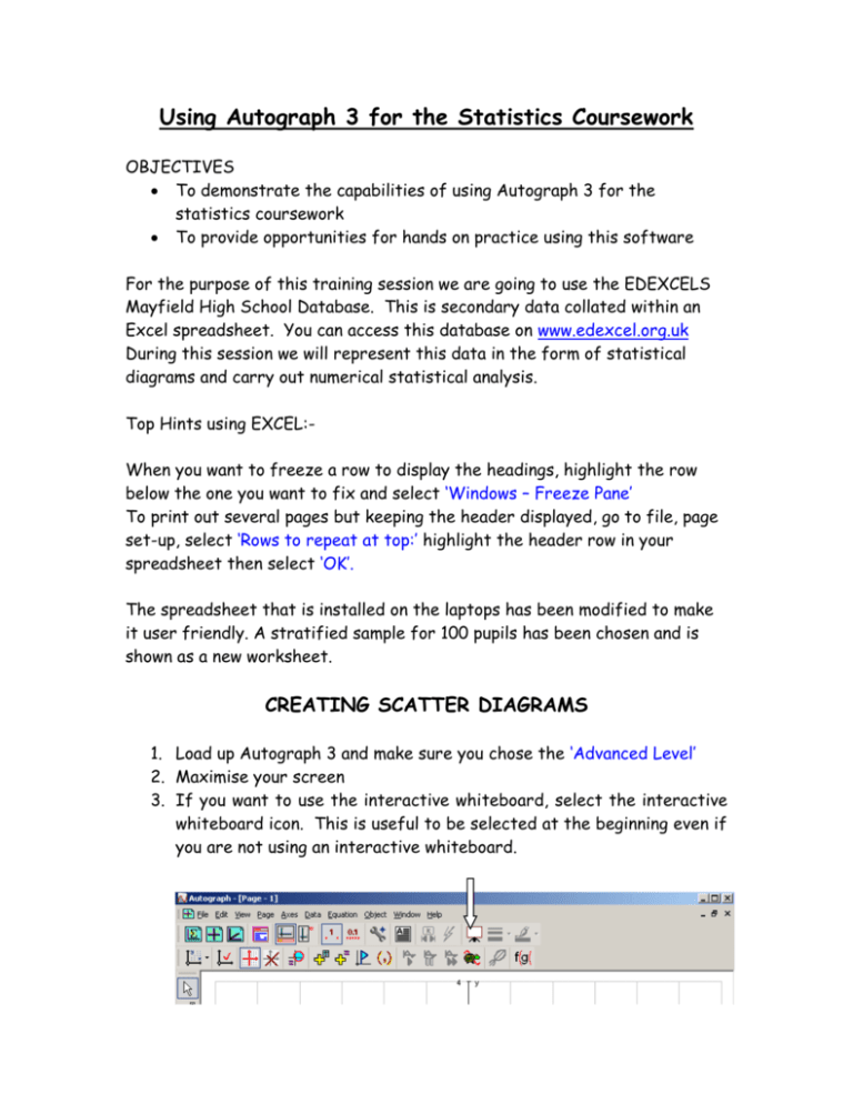
Using Autograph 3 for the Statistics Coursework
OBJECTIVES
 To demonstrate the capabilities of using Autograph 3 for the
statistics coursework
 To provide opportunities for hands on practice using this software
For the purpose of this training session we are going to use the EDEXCELS
Mayfield High School Database. This is secondary data collated within an
Excel spreadsheet. You can access this database on www.edexcel.org.uk
During this session we will represent this data in the form of statistical
diagrams and carry out numerical statistical analysis.
Top Hints using EXCEL:When you want to freeze a row to display the headings, highlight the row
below the one you want to fix and select ‘Windows – Freeze Pane’
To print out several pages but keeping the header displayed, go to file, page
set-up, select ‘Rows to repeat at top:’ highlight the header row in your
spreadsheet then select ‘OK’.
The spreadsheet that is installed on the laptops has been modified to make
it user friendly. A stratified sample for 100 pupils has been chosen and is
shown as a new worksheet.
CREATING SCATTER DIAGRAMS
1. Load up Autograph 3 and make sure you chose the ‘Advanced Level’
2. Maximise your screen
3. If you want to use the interactive whiteboard, select the interactive
whiteboard icon. This is useful to be selected at the beginning even if
you are not using an interactive whiteboard.
4. Now you are ready to enter the two sets of data from Excel.
Minimise the Autograph 3 page and open up your Mayfield
spreadsheet. Open the worksheet named SAMPLE BOYS AND GIRLS.
If we are testing a hypothesis with relation to heights and weights,
we need to highlight these two columns and select edit-copy. Minimise
Excel and maximize Autograph 3.
5. Select the icon ‘Enter XY Data Set….’
6. Before you paste your data into Autograph 3, select ‘Use x-header as
x-axis label’ and ‘Use y-header as y-axis label’. Also select ‘Show
statistics’ and name your data set. Now paste your data into the x, y
columns. Two ways you can do this. ‘Ctrl +V’, or right click on your
mouse and select ‘paste’. Before you select OK, you need to ‘Sort by
x’ and ‘Sort by y’ to ensure that there are no obvious anomalies in the
secondary data. If there are you can delete them.
7. Now click ‘OK’. A scatter diagram will appear along with statistics
results. The software will prompt you to transfer these to a results
box, select this and close down the statistics results. You will also
need to change the axes from the default scales you can select the
spanner icon or follow these prompts. ‘Axes – Edit Axes’ and alter the
minimum and maximum x, y values. You could right click on your mouse
and select ‘Edit Data Set’ and ‘Sort by x’, ‘Sort by y’, to find the range
of your data
8. If you want to add a title you can do this by selecting the text box
icon (located to the right of the spanner icon)
9. To improve the appearance of the graph, you can do a variety of
things. Here is a typical example ‘Axes - Edit Axes - Appearance Theme Preferences: Graph Paper – OK’. To remove the prompt bar at
the bottom of the screen ‘Axes - Edit Axes - Options - Key: None’
10. To add a line of best fit ‘Edit – Select All’ then right-click on the
mouse and select ‘Best Fit’ and select ‘Polynomial order 1’. An
alternative method would be to select ‘y on x regression line’. At the
bottom of your screen you will find the equation of this line, double
click on this label bar and this will appear magnified at the top of your
page. If you select the text box, you can copy and paste this text
into your text box, then play around with the font to make it colourful
etc
11. EXTENSION – Using the worksheets in your Mayfield spreadsheet
can you create two scatter diagrams on one page, showing boys’
heights against boys’ weights and girls’ heights against girls’ weights
along with all the appropriate statistics? To view these statistics
select view, results box, or use the shortcut icon, can you find it????
CREATING BOX AND WHISKER DIAGRAMS
We will create a box and whisker diagram using Autograph 3, from a set of
raw data created in the Mayfield spreadsheet. Before we start we need to
open the statistics page in Autograph 3.
‘File – New 1D Statistics Page’, or double clip on the sigma icon.
Minimise the screen and open up the Mayfield spreadsheet.
We will begin by plotting a box and whisker diagram for the boys’ heights.
To do this highlight the column needed and select ‘Edit – Copy’, or ‘CTRL +C’,
and minimise the spreadsheet. Maximise Autograph 3.
If you run your mouse along the four yellow crosses, you will find out their
function. One should read ‘Enter Raw Data… ‘Select this cross and then
paste your data in from Excel, right click on the mouse and choose ‘Paste’, or
‘CTRL +V’. Your data is now entered and you can sort the data to ensure that
there are no anomalies. Once you are happy with the set of data, select the
box and whisker icon and select ‘OK’.
A box and whisker diagram will appear. You can alter the x-axis and change
the scale. To change the intervals, ‘Axes - Edit Axes – Spacing’, deselect
the Auto on the x-axis and change the x-pips to 0.01, this will enable the
students to read the quartiles. Autograph 3 actually does the statistical
analysis for you.
To view the results you need to select the sigma icon for the statistics
results and then transfer them into the results box, which is located next to
the statistics results
If you double click on the bar at the bottom of you screen you can use part
of this as text.
Pupils can then save this as a screen saver ‘Ctrl Prt Sc’ or ‘Page, Copy Page’,
or ‘Ctrl +C’. They can then begin to interpret their results.
Autograph 3 enables you to have more than one box and whisker diagram on
a page at the same time. This is extremely useful when comparing two sets
of data. To do this, follow the same procedure as before but move the new
box and whisker around the page vertically using the mouse. Make sure the
new box and whisker diagram is also labeled.
Extension, create a box and whisker diagram for the girls’ heights on the
same page.
The third yellow cross allows you to create a box and whisker diagram using
known parameters.
CREATING A FREQUENCY DIAGRAM (HISTOGRAM)
This can be done in two ways


Entering raw data and allowing the software to group the data to
create a frequency diagram
Entering data manually from a frequency table, this allows you to
create histograms with unequal widths
To enter the raw data, you need to select the first yellow cross, ‘Enter
Grouped Data’. Rename the data set with Boys Heights. Enter the Max and
Min values, these only need to be an estimate, and alter the class width to
0.1. You can change this later. Select ‘Use Raw Data’ under Frequencies,
select ‘Edit’, and then paste in your boys’ heights. Select ‘OK’, and then ‘OK’
again to select continuous data. Now you can select the frequency diagram
(histogram) icon and select ‘OK’. You might need to change your axes or
alter the width of your bars. You can do this by Editing the Data Set (Right
click – ‘Edit Data Set’). Autograph 3 will put in a default class width, in this
case 0.4, despite the fact that we entered 0.1. Go back to the data set and
change this.
Can you repeat this for Girls’ Heights and try and plot them back to back, by
selecting ‘Plot Up’ or ‘Plot Down’