EXPLORATION
TECHNOLOGY
Originally appeared in:
January 2009 issue, pgs 61-66.
Posted with permission.
Removing surface-related
multiples just got better
A new multiple subtraction method uses the
attributes of predicted multiples, not the multiples themselves.
Manhong Guo, Young Kim, Satyakee Sen, Jim Xu,
Jing Xie and Bin Wang, TGS-NOPEC Geophysical Company
Multiple reflections of seismic waves namely, dip and Average Absolute Value convolution-based prediction1 and
off of the seafloor have been keeping (AAV) along the dip. Instead of subtract- wavefield-extrapolation-based predicprocessing experts busy for years. To get ing adapted or matched multiples, the tion2—were compared and well suma clear image of the subsurface, the true subtracted multiples are directly estimat- marized by Matsen and Xia.3 Both preor primary seismic reflection must be ed from the data using the dip and AAV diction methods can accurately predict
preserved while the multiple reflections of the predicted multiples. This method the timing of multiples. However, they
are removed—no easy task. Remov- eliminates the complicated matching step are not ideal because they both alter the
ing surface-related diffracted multiples and provides a more accurate preservation waveform of multiples.
in 3D seismic data is a challenging but of the primary reflections. We have tested
Convolution-based approaches change
necessary process to ensure accurate this method on field data, and the results the waveform by doubling the source
have been that the new method removed wavelet spectrum in the frequency doevent placement.
One solution that has seen substantial the multiples while preserving the prima- main. In addition, interpolated traces are
progress is the use of predicted multiples ries better than conventional adaptive- used to generate missing source-receiver
to subtract the surface-related multiples. subtraction methods.
pairs at the bounce points under the waThere have been some excellent techniques
ter surface, and these traces may not have
developed for predicting multiples, such MULTIPLE SUBTRACTION
the same waveform as the missing traces.
as convolution-based or wavefield-extrap- METHODS
Wavefield-extrapolation-based apolation-based approaches. However, diffiFor background, the two common proaches also change the waveform; the
culty stems from the fact that many exist- approaches for predicting multiples— only way to avoid this is to use a pering techniques try to match the
fect reflectivity model, which
predicted multiples to the mulis impractical to obtain. These
Data: primaries
Predicted
tiples in the data by either adwaveform changes make suband multiples
multiples
aptation or pattern matching.
tracting multiples in the data
Dip scan
Dip scan
The issue with these prediction
using the predicted multiples a
techniques is that they change
challenging task.
Pp, Ap and Pm, Am
Pm, Am
the waveform of the predicted
One common approach
multiples, and this makes it
for subtracting multiples using
very difficult to perfectly match
predicted multiples is adaptive
Pp
the waveform of the predicted
subtraction.4 Adaptive subtracmultiples to that of the multion tries to match the wavetiples in the data.
form of the predicted multi+
Estimated
Estimated
–
The R&D team at the auprimaries
ples to that in the data in both
multiples
thors’ company realized that
amplitude and phase in a winthe matching process was alterdow. This technique provides
Residual primaries
and multiples
ing the data in such a way that
cause for concern for a couple
multiple subtraction was really
of reasons. First, if the window
not as reliable as it could be.
is small enough to include only
+ –
Our solution was to develop a
multiples, the window may not
new technique for subtracting
be able to provide enough stamultiples without the matchtistics to design a reliable filter.
Primaries
ing process that could provide
Conversely, if the window is
Fig. 1. The new method uses dip and Average Absolute Value
more accurate results.
large, it may contain primaries
The new approach simplifies of the data events and in the predicted multiples. Step 1
and other noise to limit the adthe multiple subtraction process determines whether a given sample in the data belongs to
aptation process.
primary or a multiple. Step 2 estimates the multiples and
by only using specific attributes asubtracts
Another approach to multhem.
of the predicted multiples,
tiple subtraction is based on
JANUARY 2008 World Oil
EXPLORATION TECHNOLOGY
pattern matching.5 One designs a Prediction Error Filter (PEF) for the primary by
deconvolving the PEF of the data with
that of the predicted multiples. Comparison of adaptive subtraction versus pattern
matching is well-documented by Abma
et al.6 They report that a pattern-matching technique also has its disadvantages.
This method tends to leave much residual multiple energy and to weaken the
primaries where the predicted multiples
overlapped the primaries.
step. Using the dip of the events in the
predicted multiples, the multiples from
the new data set are estimated or reconstructed by averaging over a few traces
along the dip of the multiples. These estimated multiples are subtracted from the
data. Reconstructing the multiples using
the data set from which most primaries
are removed allows for more reliable estimation of the multiples in the data.
Note that, instead of generating a filter that will try to match the predicted
multiples to the multiples in the data,
the multiples in the data are directly deNEW MULTIPLE SUBTRACTION
termined using the dip of the predicted
METHOD
multiples. In other words, the predicted
The new approach developed by the
multiples are used only to determine the
authors avoids the matching process aldip of the multiples in the data. In doing
together, which may have been the main
so, one can avoid the step of matching
source of difficulty in previous approachthe waveform of the predicted multiples
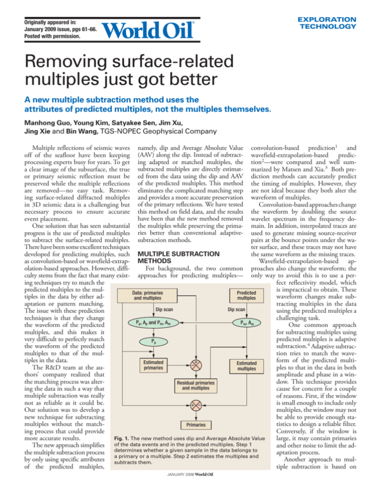
es. Figure 1 shows a flow diagram of the
to that of the multiples in the data.
new method using the dip and AAV of
Figure 2a shows a common offset synthe events in the data and in the predictthetic data set that contains two flat, pried multiples. It consists of two steps. The
mary events and one primary diffraction
first step is to determine whether a given
indicated by P and white arrows and their
sample in the data belongs to a primary
multiples. Figure 2b displays the predictor a multiple. In the second step, the
ed multiples using wavefield extrapolamultiples in the data are estimated and
tion. Basically, a round trip was added to
subtracted from the data.
each depth in the migrated section (not
The dip scan is used to determine the
shown). Note that the waveform of the
dip of the events in the data that contains
predicted multiples is different from that
primaries, multiples and other noises.
of the data. By comparing the dip and
The dip scan is also used to determine
AAV of the event in the data and those of
the dip of the events in the predicted
the corresponding event in the predicted
multiples. Next, the dip of the events in
Fig. 2. a) A common offset section,
multiples, the primaries and their dip
b) the predicted multiples and c) the
the data is compared with the dip of the
reconstructed multiples.
can be identified. The primaries are estievents in the predicted multiples to sepamated by averaging over a few
rate the dip of the primaries.
traces along the dip in the data
If the dip at a sample point in
and subtracting them from the
the data is sufficiently different
data. This step results in a new
from the dip at the same samdata set that mostly contains
ple location in the predicted
the multiples in the data. This
multiples, the sample in the
data set is used to determine
data is considered as a primary.
the multiples by averaging over
On the other hand, if they are
a few traces along the dip of
similar, then that sample in the
the multiples.
data is considered a multiple.
Using the data set that
In addition, the AAV is anmostly contains the multiples
other criterion used to distinprovides an advantage over usguish the primaries from the
ing the original data set for demultiples, particularly when
termining the multiples. Since
the dips are similar. Because
the original data includes the
of spurious noises in the preprimaries or other noises, averdicted multiples, the dip at a
aging over a few traces along a
sample point in the predicted
multiple dip can be affected by
multiples can be similar to that
the primaries or other noises.
of the sample at the same loFigure 2c shows the estimated
cation in the data. However,
multiples that will be subthe AAV along the dip in the
tracted from the data. Note
predicted multiples should be
that the waveform of the estimuch smaller than the AAV
mated multiples is the same as
along the same dip in the data. Fig. 3. Synthetics: a) subtraction using the attributes of the
predicted multiples, and b) conventional adaptive subtraction.
the waveform of the multiples
In such cases, the sample is re- Note the residual multiples (white arrow) and in the ellipse.
in the data. The white arrows
garded as a primary.
In the second step, assuming the
waveform does not change much over
a few traces, the primaries are estimated
by averaging over a few traces along the
dip. Then the estimated primaries are
subtracted from the data to obtain a new
data set that contains all the multiples.
The new data set may also contain some
residual primaries that were not properly
accounted for in the previous estimation
JANUARY 2008 World Oil
EXPLORATION TECHNOLOGY
in Fig. 2 indicate a) the multiple in the
data, b) the predicted multiple and c) the
reconstructed multiple.
Figure 3a shows the result of subtracting the estimated multiples from
the data. Note that all the multiples are
subtracted properly. Figure 3b displays
the result of adaptive subtraction. The
flat primary where a diffracted multiple
coincides with the primary in the data is
distorted. There is a difference between
the waveform of the predicted multiples
and the waveform of the data where the
primary and the diffracted multiple are
overlapped. This difference prevents adaptation from perfectly fitting only the
multiples in the data. In addition, a noticeable amount of multiple energy is left
after adaptive subtraction (indicated by a
white arrow).
ed by the water surface and any reflectors down to the depth of 3,000 m. Note
that the location of predicted multiples is
precise, but the waveform of the predicted multiples is quite different from the
waveform of the multiples in the data.
Figure 4c shows the result after subtracting the multiples using the new
method. Note that the first-order waterbottom multiples and their peg legs are
well suppressed. After subtracting the
multiples, many steeply dipping primary
events, as well as gently dipping reflections (see the events inside the ellipse),
are well-retained, which were previously
masked by high-amplitude multiples.
For comparison, we used an adaptive
subtraction method and displayed the
results in Fig. 4d. The subtraction was
somewhat mild to preserve the primaries. As a result, a noticeable amount of
multiple energy was left. Many steeply
or gently dipping primary events are still
masked by residual multiples. If the adaptation parameters are tightened, more
multiples can be subtracted, but some
primaries could also be removed.
Shown in Fig. 5 are the spectra of the
data shown in Fig. 4. The green curve
shows the spectrum of the input data,
the red curve shows the spectrum of the
adaptive subtraction, and the brown
curve shows the spectrum of the attribute-based subtraction. The notch in
the input spectrum is due to towing the
streamer at a depth of 18 m to retain the
low-frequency components of the data.
These spectra illustrate the performance
of the two subtraction techniques. The
adaptive subtraction method failed to
match the predicted multiples to the
multiples in the data in the high-frequency range. Basically, there was no
subtraction of high-frequency components. On the other hand, the attributebased subtraction worked well on all
frequency components.
Amplitude, dB
RESULTS
Figure 4a shows a common offset
section of an inline from a marine 3D
survey. The data were acquired using six
streamers of 9-km length with a cable
spacing of 160 m in the deepwater Gulf
of Mexico. Because of severe feathering,
each shot gather had to be regularized
on a uniform grid with an inline spacing
of 12.5 m and a crossline spacing of 80
m. A preliminary depth-migrated cube
was used as a reflectivity model and the
corresponding velocity model was used
as a velocity model for wavefield extrapolation to predict the multiples. To
prevent wraparound noises, the computation grid was extended. The nominal
distance of the computation grid in the
crossline direction was 4 km. Because
of severe feathering, a computation grid
CONCLUSIONS
wider than 8 km in the crossline direcAdaptive subtraction approaches
tion was used for some shots. About 6
have been a main tool for subtracting
Fig. 4. a) Input, b) predicted multiples,
km in the inline direction was also padthe predicted multiples from the data.
c) attribute-based subtraction and d)
ded to avoid wraparound noises in the
However, matching can be either too
adaptive subtraction.
inline direction.
aggressive or too mild. When it is too
The difference between
aggressive, the multiples can
the dip of the primaries and
be eliminated, but many prithe dip of multiples is more
maries are also partially re0
evident in the common offset
moved. On the other hand,
domain than in the common
when matching is too mild,
shot domain. For this reason,
most primaries are preserved,
the method was applied in the
but much of the multiple encommon offset domain. Figure
-10
ergy also remains.
4b shows the predicted multiA new method using the
ples by extrapolating the shot
attributes of the data and pregathers to a depth of 3,000 m,
dicted multiples avoids the
which is deeper than the deepmatching of the predicted
est top of the salt, and back to
multiples to the multiples in
-20
0
40
80
the surface. This depth ensures
the data. Instead, it uses the
Frequency, Hz
that wave field extrapolation
dip and AAV at each sample
can predict both source- and Fig. 5. Amplitude spectra of the data shown in Fig. 4.
in the data and in the predictreceiver-side multiples bounded multiples to differentiate
JANUARY 2008 World Oil
EXPLORATION TECHNOLOGY
the primaries from the multiples. Once
it is identified as a primary, the primary
is estimated as an average of the samples
along the dip over a few traces.
These estimated primaries are subtracted from the data to make a new
data set, from which the multiples are
estimated by summing over a few traces
along the dip of the multiples.
The new method works well for most
multiples except when a primary and
a multiple overlap each other with the
same dip and a similar AAV. For example, a flat primary and the apex of diffracted multiples can overlap with a flat
dip. In such cases, one may determine
the dip by scanning over a large number
of traces such that the AAV of the primary will be much higher than that of
the diffracted multiples.
The current tests on field data show
favorable results for the new method;
the multiples were removed and primaries were preserved better than conventional adaptive subtraction methods.
The R&D team plans to continue improving the methodology by exploring
some other attributes, such as frequency, which could help further separate
primaries from multiples. The team is
exploring the possibility of combining
this method with the traditional adaptive subtraction process. These new
techniques will continue to be tested
and eventually implemented, along
with many other efficiency-improving
methods for clarifying subsurface images. WO
a part of TGS-NOPEC Geophysical Company,
where he is a Senior Research Geophysicist.
ACKNOWLEDGMENTS
The authors would like to thank James Cai and
Zhiming Li for their technical input and Shannon
Morolez for editing.
Satyakee Sen received an MS degree in geophysics from Pennsylvania State University.
He joined TGS-NOPEC Geophysical Company
in 2006 and has been conducting research on
multiple estimation and suppression. He is a
Research Geophysicist.
LITERATURE CITED
D. J., Berkhout, A. J. and C. P. A. Wapenaar, “Adaptive surface-related multiple subtraction,” Geophysics, 57, 1992, pp.
1,166–1,177.
2Pica, A., et al., “3-D surface-related multiple modeling, principles
and results,” Society of Exploration Geophysicists, Expanded Abstracts, 2005, pp. 2,080–2,083.
3Matsen, K. and G. Xia, “Multiple attenuation methods for wide
azimuth marine seismic data,” Society of Exploration Geophysicists,
Expanded Abstracts, 2007, pp. 2,476–2,479.
4Verschuur, D. J., Berkhout, A. J. and C. P. A. Wapenaar, “Adaptive surface-related multiple subtraction,” Geophysics, 57, 1992, pp.
1,166–1,177.
5Spitz, S., “Pattern recognition, spatial predictability, and subtraction
of multiple events,” The Leading Edge, 18, 1999, pp. 55–58.
6Abma, R., et al., “Comparisons of adaptive subtraction methods for
multiple attenuation,” The Leading Edge, 24, 2005, pp. 277–280.
1Verschuur,
The authors
Manhong Guo received an MS degree in computer science from the University of Houston and
in geology from the Institute of Geology, China.
In 2001 he joined NuTec Energy, which became
Article copyright © 2009 by Gulf Publishing Company. All rights reserved.
Young Kim is Chief Scientist at TGS-NOPEC.
He earned a PhD degree in electrical engineering from the University of Texas at Austin.
Upon retiring from ExxonMobil, he joined TGSNOPEC Geophysical Company to build a new
R&D team in 2005.
Jim Xu received his PhD degree in aerospace
engineering from the University of Texas at
Austin. Jim worked for Atmospheric & Environmental Research, Inc., and Shell International
E&P. He joined TGS-NOPEC Geophysical Company in 2005 to conduct research in multiple
estimation and suppression. He is currently a
Processing Geophysicist.
Jing Xie worked for WesternGeco and GeoTomo and joined TGS-NOPEC Geophysical in
2005, where he is a Senior Software Engineer.
He earned his PhD degree in petroleum engineering from the University of Texas at Austin.
Bin Wang earned a PhD degree in geophysics
from Purdue University in 1993, and an MBA
from Southern Methodist University in 2001.
He started his career with Mobil Oil in 1993,
and joined TGS-NOPEC in March 2007. He is
now general manager of R&D at TGS-NOPEC.
Printed in U.S.A.
Not to be distributed in electronic or printed form, or posted on a website, without express written permission of copyright holder.