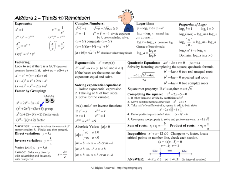
Algebra 2 – Things to Remember!
Exponents:
x0 1
x m • x n x m n
m
x
x mn
n
x
1
xm m
x
n m
( x ) x n• m
n
x
x
n
y
y
n
( xy ) n x n • y n
Factoring:
Look to see if there is a GCF (greatest
common factor) first. ab ac a (b c)
x 2 a 2 ( x a )( x a)
( x a) 2 x 2 2ax a 2
( x a) 2 x 2 2ax a 2
Factor by Grouping:
proportionality, k. Find k, and then proceed.
with advertising and inversely
with candy cost.
by 4, use remainder, solve.
ka
y
c
Logarithms
y log b x x b y
ln x log e x natural log
Properties of Logs:
log b b 1
log b 1 0
e = 2.71828…
m
log b log b m log b n
n
log b (m r ) r log b m
Domain: log b x is x 0
(a bi ) conjugate (a bi )
(a bi )(a bi ) a 2 b 2
Change of base formula:
a bi a 2 b 2 absolute value=magnitude
log b a
Exponentials e x exp( x)
b x b y x y (b 0 and b 1)
If the bases are the same, set the
exponents equal and solve.
Solving exponential equations:
1. Isolate exponential expression.
2. Take log or ln of both sides.
3. Solve for the variable.
Variation: always involves the constant of
Direct variation: y kx
k
Inverse variation: y
x
Varies jointly: y kxj
Combo: Sales vary directly
Complex Numbers:
1 i
a i a ; a 0
2
14
i 1
i i 2 1 divide exponent
log x log10 x common log
log a
log b
Quadratic Equations: ax 2 bx c 0 (Set = 0.)
Solve by factoring, completing the square, quadratic formula.
b 2 4ac 0 two real unequal roots
2
b b 4ac
x
b 2 4ac 0 repeated real roots
2a
b 2 4ac 0 two complex roots
Square root property: If x 2 m, then x m
Completing the square:
x2 2 x 5 0
1. If other than one, divide by coefficient of x2
2. Move constant term to other side x 2 2 x 5
3. Take half of coefficient of x, square it, add to both sides
x2 2x 1 5 1
ln( x) and e x are inverse functions
ln e x x
eln x x
ln e 1
eln 4 4
2
e 2ln 3 eln 3 9
4. Factor perfect square on left side.
Absolute Value: a 0
Sum of roots: r1 r2
a; a 0
a
a; a 0
m b m b or m b
m b b m b
log b (mn) log b m log b n
( x 1) 2 6
5. Use square root property to solve and get two answers. x 1 6
b
c
Product of roots: r1 r2
a
a
2
Inequalities: x x 12 0 Change to =, factor, locate
critical points on number line, check each section.
(x + 4)(x - 3) = 0
x = -4; x = 3
m b m b or m b
ANSWER: -4 < x < 3 or [-4, 3] (in interval notation)
All Rights Reserved: http://regentsprep.org
Radicals: Remember to use fractional exponents.
a
n
xx
an a
1
a
m
n
x n xm
n
ab n a n b
n
x
n
m
a na
b nb
Simplify: look for perfect powers.
x12 y17 x12 y16 y x 6 y 8 y
72 x 9 y 8 z 3 3 89 x 9 y 6 y 2 z 3 2 x3 y 2 z 3 9 y 2
Use conjugates to rationalize denominators:
5
2 3
10 5 3
10 5 3
2 3 2 3 42 3 2 3 9
Equations: isolate the radical; square both sides
to eliminate radical; combine; solve.
2 x 5 x 3 0 (2 x 3) 2 (5 x ) 2
3
4 x 2 12 x 9 25 x solve : x 9; x 1/ 4
CHECK ANSWERS. Answer only x = 9.
Functions: A function is a set of ordered pairs in which
each x-element has only ONE y-element associated with it.
Vertical Line Test: is this graph a function?
Domain: x-values used; Range: y-values used
Onto: all elements in B used.
1-to-1: no element in B used more than once.
Composition: ( f g )( x) f ( g ( x))
Inverse functions f & g: f ( g ( x)) g ( f ( x)) x
Horizontal line test: will inverse be a function?
Transformations:
f ( x) over x-axis; f ( x) over y-axis
f ( x a) horizontal shift; f ( x) a vertical shift
f (ax) stretch horizontal; af ( x) stretch vertical
Working with Rationals ( Fractions):
Simplify:
remember to look for a factoring of -1:
3 x 1 1( 3 x 1 )
1
1 3x
1 3x
Add: Get the common denominator.
Factor first if possible:
Multiply and Divide: Factor First
Rational Inequalities
x 2 2 x 15
0 The critical values
x2
from factoring the numerator are -3, 5.
The denominator is zero at x = 2.
Place on number line, and test sections.
Sequences
Arithmetic: an a1 (n 1)d
n(a1 an )
Sn
2
n 1
Geometric: an a1 r
a1 (1 r n )
1 r
Recursive: Example:
a1 4; an 2an 1
Sn
Binomial Theorem:
n
n
(a b) n a n k b k
k 0 k
Solving Rational Equations:
Get rid of the denominators by mult. all terms by
common denominator.
22
3
2
2
2x 9x 5 2x 1 x 5
multiply all by 2 x 2 9 x 5 and get
22 3( x 5) 2(2 x 1)
22 3x 15 4 x 2
37 3x 4 x 2
35 7 x
5 x
Great! But the only problem is that
x = 5 does not CHECK!!!! There is no solution.
Extraneous root.
Motto: Always CHECK ANSWERS.
Equations of Circles: x 2 y 2 r 2 center origin
( x h) 2 ( y k ) 2 r 2 center at (h,k)
x 2 y 2 Cx Dy E 0 general form
Complex Fractions:
Remember that the fraction bar means divide:
Method 1: Get common denominator top and bottom
2 4 2 4x
1
2
x2 x x2 2 4 x 4 x 2 2 4 x x
1
4 2
4x 2
x2
x2
4x 2
x2
2
x x
x2
Method 2: Mult. all terms by common denominator for
all.
2 4
2
4
x2 2 x2
2
x
x
x
x 2 4 x 1
4 2
4
2
4x 2
2
x2 x2 2
x x
x
x
All Rights Reserved: http://regentsprep.org
Trigonometry –
Things to Remember!
Radians and Degrees
Arc Length of a Circle = r (in radians)
Change to degrees multiply by
Special Right Triangles
Quadrantal angles – 0, 90, 180, 270
Change to radians multiply by
180
180
CoFunctions: examples
sin cos(90º ) ; tan cot(90º )
30º-60º-90º triangle
side opposite 30º = ½ hypotenuse
side opposite 60º = ½ hypotenuse
3
45º-45º-90º triangle
Inverse notation:
arcsin(x) = sin-1(x)
arccos(x) = cos-1(x)
arctan(x) = tan-1(x)
Trig Functions
o
a
o
sin ; cos ; tan
h
h
a
h
h
a
csc ; sec ; cot
o
a
o
Reciprocal Functions
1
1
1
sin
; cos
; tan
csc
sec
cot
1
1
1
csc
; sec
; cot
sin
cos
tan
tan
sin
cos
Trig Graphs
sin x
hypotenuse = leg 2
leg = ½ hypotenuse 2
Law of Sines: uses 2 sides and 2 angles
sin A sin B sin C
Has an ambiguous case.
a
b
c
cot
cos
sin
cos x
sinusoidal curve = any curve expressed as
y = A sin(B(x – C)) + D
Law of Cosines: uses 3 sides and 1 angle
c 2 a 2 b 2 2ab cos C
amplitude (A) = ½ | max – min| (think height)
Area of triangle: A = ½ ab sin C
Area of parallelogram: A = ab sin C
period = horizontal length of 1 complete cycle
Pythagorean Identities:
sin 2 cos 2 1 tan 2 1 sec 2
1 cot 2 csc2
horizontal shift (C) – movement left/right
frequency (B) = number of cycles in 2 (period)
vertical shift (D) – movement up/down
All Rights Reserved: http://regentsprep.org
Statistics and Probability –
Things to Remember!
Normal Distribution and Standard Deviation
Statistics:
x1 x2 ... xn 1 n
xi
n
n i 1
median = middle number in ordered data
mode = value occurring most often
mean x
range = difference between largest and smallest
mean absolute deviation (MAD):
1 n
population MAD xi x
n i 1
variance:
population variance ( x) 2
n
1
2
xi x
n i 1
standard deviation:
population standard deviation =
x
1 n
2
xi x
n i 1
Empirical Probability
# of times event E occurs
P( E )
total # of observed occurrences
Binomial Probability
r
nr
“exactly” r times
n Cr • p • q
n
or • p r • (1 p ) n r
r
[TI Calculator: binompdf(n, p, r)]
When computing "at least" and "at most"
probabilities, it is necessary to consider, in
addition to the given probability,
• all probabilities larger than the given
probability ("at least")
[TI Calculator: 1 – binomcdf(n, p, r-1)]
Sx = sample standard deviation
x = population standard deviation
Probability
Permutation: without replacement
and order matters
n!
n Pr
(n r )!
Combination: without replacement
and order does not matter
n n Pr
n!
n Cr
r r ! r !(n r )!
• all probabilities smaller than the given
probability ("at most")
[TI Calculator: binomcdf(n, p, r)]
Theoretical Probability
n( E )
# of outcomes in E
P( E )
n( S ) total # of outcomes in S
P(A and B) = P(A)•P(B)
for independent events
P(A and B) = P(A)•P(B| A)
for dependent events
P(A’ ) = 1 – P(A)
P(A or B) = P(A) + P(B) – P(A and B)
for not mutually exclusive
P(A or B) = P(A) + P(B)
for mutually exclusive
P ( B | A)
All Rights Reserved: http://regentsprep.org
P( A and B)
(conditional)
P( A)
