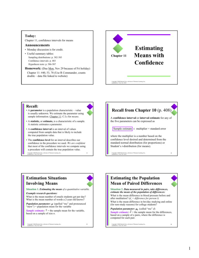
Today:
Chapter 11, confidence intervals for means
Announcements
• Monday discussion is for credit.
• Useful summary tables:
Chapter 11
Sampling distributions: p. 382-383
Confidence intervals: p. 483
Hypothesis tests: p. 586-587
Estimating
Means with
Confidence
Homework: (Due Mon, Nov 29 because of Fri holiday)
Chapter 11: #40, 53, 78 (Use R Commander, counts
double – data file linked to website)
Copyright ©2004 Brooks/Cole, a division of Thomson Learning, Inc.,
modified by J. Utts, Nov 2010
Recall:
Recall from Chapter 10 (p. 408)
• A parameter is a population characteristic – value
is usually unknown. We estimate the parameter using
sample information. Chapter 11: C.I.s for means.
A confidence interval or interval estimate for any of
the five parameters can be expressed as
• A statistic, or estimate, is a characteristic of a sample.
A statistic estimates a parameter.
Sample estimate ± multiplier × standard error
• A confidence interval is an interval of values
computed from sample data that is likely to include
the true population value.
where the multiplier is a number based on the
confidence level desired and determined from the
standard normal distribution (for proportions) or
Student’s t-distribution (for means).
• The confidence level for an interval describes our
confidence in the procedure we used. We are confident
that most of the confidence intervals we compute using
a procedure will contain the true population value.
Copyright ©2004 Brooks/Cole, a division of Thomson Learning, Inc.,
modified by J. Utts, Nov 2010
3
Copyright ©2004 Brooks/Cole, a division of Thomson Learning, Inc.,
modified by J. Utts, Nov 2010
4
Estimation Situations
Involving Means
Estimating the Population
Mean of Paired Differences
Situation 1. Estimating the mean of a quantitative variable.
Situation 2. Data measured in pairs, take differences,
estimate the mean of the population of differences:
What is the mean difference in blood pressure before and
after meditation? (di = difference for person i)
What is the mean difference in hrs/day studying and online
(for non-study reasons) for college students?
Example research questions:
What is the mean number of emails students get per day?
What is the mean number of words a 2-year old knows?
Population parameter: µ (spelled “mu” and pronounced
“mew”) = population mean for the variable
Sample estimate: x = the sample mean for the variable,
based on a sample of size n.
Copyright ©2004 Brooks/Cole, a division of Thomson Learning, Inc.,
modified by J. Utts, Nov 2010
Population parameter: µd (called “mu” d)
Sample estimate: d = the sample mean for the differences,
based on a sample of n pairs, where the difference is
computed for each pair.
5
Copyright ©2004 Brooks/Cole, a division of Thomson Learning, Inc.,
modified by J. Utts, Nov 2010
6
1
Difference in two means
Recall from Chapter 10 (p. 408)
Situation 3. Estimating the difference between two
populations with regard to the mean
of a quantitative variable.
Example research questions:
How much difference is there in average weight loss for
those who diet compared to those who exercise to lose
weight?
How much difference is there in the mean IQs for children
whose moms smoked and didn’t during pregnancy?
Population parameter: µ1 – µ2 = difference between the
two population means.
Sample estimate: x1 − x2 = difference between the two
sample means. This requires independent samples.
Copyright ©2004 Brooks/Cole, a division of Thomson Learning, Inc.,
modified by J. Utts, Nov 2010
A confidence interval or interval estimate for any of
the five parameters can be expressed as
Sample estimate ± multiplier × standard error
where the multiplier is a number based on the
confidence level desired and determined from the
standard normal distribution (for proportions) or
Student’s t-distribution (for means).
7
Rough Definition: The standard error of a
sample statistic measures, roughly, the average
difference between the statistic and the population
parameter. This “average difference” is over all
possible random samples of a given size that can
be taken from the population.
Technical Definition: The standard error of a
sample statistic is the estimated standard deviation
of the sampling distribution for the statistic.
9
In practice, the population standard deviation σ is rarely
known, so we cannot compute the standard deviation of x ,
σ
s.d.( x ) =
.
n
In practice, we only take one random sample, so we only have
the sample mean x and the sample standard deviation s.
Replacing σ with s in the standard deviation expression gives
us an estimate that is called the standard error of x .
s
s.e.( x ) =
.
n
From Chapter 9 example of a sample of n = 25 weight losses,
the sample standard deviation is s = 4.74 pounds.
So the standard error of the mean is 4.74/5 = 0.948 pounds.
Copyright ©2004 Brooks/Cole, a division of Thomson Learning, Inc.,
modified by J. Utts, Nov 2010
10
Standard Error of a Sample Mean
Increasing the Size of the Sample
Suppose we take n = 100 people instead of just 25.
The standard deviation of the mean would be
s.e.( x ) =
σ
5
=
= 0.5 pounds.
s.d.( x ) =
n
100
s
, s = sample standard deviation
n
Example 11.2 Mean Hours Watching TV
• For samples of n = 25,
sample means are likely to
range between 8 ± 3 pounds
=> 5 to 11 pounds.
• For samples of n = 100,
sample means are likely to
range only between 8 ± 1.5
pounds => 6.5 to 9.5 pounds.
Poll: Class of 175 students. In a typical day, about
how much time do you spend watching television?
Minitab provides s.e., R Commander doesn’t, but provides s
Statistics → Summaries → Numerical summaries, check Standard Deviation
VariableN
Mean Median TrMean StDev
TV
175 2.09 2.000 1.950 1.644
s .e .( x ) =
Larger samples tend to result in more accurate estimates
of population values than smaller samples.
Copyright ©2004 Brooks/Cole, a division of Thomson Learning, Inc.,
modified by J. Utts, Nov 2010
8
Standard Error of the Mean
Standard errors (in general)
Copyright ©2004 Brooks/Cole, a division of Thomson Learning, Inc.,
modified by J. Utts, Nov 2010
Copyright ©2004 Brooks/Cole, a division of Thomson Learning, Inc.,
modified by J. Utts, Nov 2010
11
SE Mean
0.124
s
1 . 644
=
= . 124
n
175
Copyright ©2004 Brooks/Cole, a division of Thomson Learning, Inc.,
modified by J. Utts, Nov 2010
12
2
Standard Error of the Difference
Between Two Sample Means (unpooled)
Standard Error for the mean of
paired differences
s.e.( d ) =
sd
n
s.e.( x1 − x2 ) =
where sd = sample standard deviation for the differences
Example: How much taller (or shorter) are daughters
than their mothers these days? sd = 3.14 (for individuals)
n = 93 pairs (daughter – mother) d = 1.3 inches
s .e .(d ) =
sd
3 . 14
=
= . 33
n
93
Copyright ©2004 Brooks/Cole, a division of Thomson Learning, Inc.,
modified by J. Utts, Nov 2010
Recall from Chapter 10 (p. 408)
A confidence interval or interval estimate for any of
the five parameters can be expressed as
Sample estimate ± multiplier × standard error
Study: n1 = 42 men on diet, n2 = 27 men on exercise routine
Diet: Lost an average of 7.2 kg with std dev of 3.7 kg
Exercise: Lost an average of 4.0 kg with std dev of 3.9 kg
So, x1 − x2 = 7.2 − 4.0 = 3.2 kg
(3.7 )2 + (3.9)2
42
47
= 0.81
Copyright ©2004 Brooks/Cole, a division of Thomson Learning, Inc.,
modified by J. Utts, Nov 2010
14
Student’s t-Distribution:
Replacing σ with s
Dilemma: we generally don’t know σ. Using s we have:
t=
x−µ
x−µ
n (x − µ)
=
=
s.e.( x ) s / n
s
If the sample size n is small,
this standardized statistic will
not have a N(0,1) distribution
but rather a t-distribution with
n – 1 degrees of freedom (df).
The multiplier is a number based on the confidence
level desired and determined from the standard
normal distribution (for proportions) or Student’s tdistribution (for means).
Copyright ©2004 Brooks/Cole, a division of Thomson Learning, Inc.,
modified by J. Utts, Nov 2010
Example 11.3 Lose More Weight by Diet or Exercise?
and s.e.( x1 − x2 ) =
13
s12 s22
+
n1 n2
15
Copyright ©2004 Brooks/Cole, a division of Thomson Learning, Inc.,
modified by J. Utts, Nov 2010
16
Finding the t-multiplier
• Excel: See page 452.
• R Commander:
Distributions → Continuous distributions →
t distribution → t quantiles
–
–
–
–
–
Probabilities: α/2 (for 95%, use .025)
Degrees of freedom
Lower tail
Gives negative of the t-multiplier
Ex: .025, 25, lower tail → −2.059539, multiplier ≈ 2.06
• Table A2, page 728 (easy to use compared to z!)
17
18
3
Confidence Interval for
One Mean or Paired Data
Example: 95% C.I. for Mean Body Temperature
Data from a blood bank near Seattle (from friend of Dr. Utts).
n = 101 blood donors, ages 17 to 84 (large sample)
Sample mean = 97.89 degrees
Sample standard deviation = 0.73 degrees
A Confidence Interval for a Population Mean
x ± t * × s.e.(x ) ⇒ x ± t * ×
s
n
where the multiplier t* is the value in a t-distribution
with degrees of freedom = df = n - 1 such that the area
between -t* and t* equals the desired confidence level.
Standard error of the mean =
Multiplier = t* with df of 100 = 1.98 (from Table A.2)
(Found from Excel, R Commander or Table A.2.)
Conditions:
• Population of measurements is bell-shaped (no major
skewness or outliers) and r.s. of any size > 2; OR
• Population of measurements is not bell-shaped,
but a large random sample is measured, n ≥ 30.
Copyright ©2004 Brooks/Cole, a division of Thomson Learning, Inc.,
modified by J. Utts, Nov 2010
Sample estimate ± multiplier × standard error
97.89 ± 1.98 × 0.073
97.89 ± 0.14
97.75 to 98.03 degrees (does not cover 98.6)
19
Paired Data Confidence Interval
Population parameter: µd = mean of differences
for the population (same as µ1 – µ2).
Sample estimate: d = sample mean of the differences
Standard deviation and standard error:
sd = standard deviation of the sample of differences;
s
s.e.(d ) = d
n
Confidence interval for µd: d ± t * × s.e. d ,
( )
Copyright ©2004 Brooks/Cole, a division of Thomson Learning, Inc.,
modified by J. Utts, Nov 2010
20
Find 90% C.I. for difference:
(daughter – mother) height difference
Data: two variables for n individuals or pairs;
use the difference d = x1 – x2.
where df = n – 1 for the multiplier t*.
0.73
= 0.073
101
How much taller (or shorter) are daughters than their mothers
these days?
n = 93 pairs (daughter – mother), d = 1.3 inches
sd = 3.14 inches, so s .e .(d ) = s d = 3 . 14 = . 33
n
93
Multiplier = t* with 92 df for 90% C.I. = 1.66 (use df=90)
Sample estimate ± multiplier × standard error
1.3 ± 1.66 × 0.33
1.3 ± 0.55
0.75 to 1.85 inches (does not cover 0)
21
22
Example 11.9: Small sample, so check for outliers
Confidence interval interpretations
• We are 95% confident that the mean body
temperature for healthy adults (who would
donate blood??) is between 97.75 degrees and
98.03 degrees.
• We are 90% confident that the mean height
difference between female college students
and their mothers is between 0.75 and 1.85
inches, with students being taller than their
mothers.
23
Data: Hours spent watching TV and hours spent on
computer per week for n = 25 students.
Create a 90% CI for the
mean difference in
hours spent using
computer versus
watching TV.
Note: Boxplot shows no obvious skewness and no outliers.
Copyright ©2004 Brooks/Cole, a division of Thomson Learning, Inc.,
modified by J. Utts, Nov 2010
24
4
Example 11.9 Screen Time: Computer vs TV
Results:
d = 5.36, sd = 15.24, and s.e.(d ) =
sd 15.24
=
= 3.05
n
25
A CI for the Difference Between Two Means
Multiplier t* from Table A.2 with df = 24 is t* = 1.71
(Independent Samples, unpooled case):
90% Confidence Interval:
5.36 ± 1.71(3.05) => 5.36 ± 5.22 => 0.14 to 10.58 hours
x1 − x2 ± t *
s12 s22
+
n1 n2
where t* is the value in a t-distribution with area
between -t* and t* equal to the desired confidence
level.
Interpretation: We are 90% confident that the average
difference between computer usage and television viewing
for students represented by this sample is covered by the
interval from 0.14 to 10.58 hours per week, with more hours
spent on computer usage than on television viewing.
Copyright ©2004 Brooks/Cole, a division of Thomson Learning, Inc.,
modified by J. Utts, Nov 2010
11.4 CI for Difference Between Two
Means (Independent samples)
25
Copyright ©2004 Brooks/Cole, a division of Thomson Learning, Inc.,
modified by J. Utts, Nov 2010
Necessary Conditions
Degrees of Freedom
• Two samples must be independent.
The t-distribution is only approximately correct
and df formula is complicated (Welch’s approx):
26
Either …
• Populations of measurements both bell-shaped,
and random samples of any size are measured.
or …
Statistical software can use the above
approximation, but if done by hand then use a
conservative df = smaller of (n1 – 1) and (n2 – 1).
• Large (n ≥ 30) random samples are measured.
27
Copyright ©2004 Brooks/Cole, a division of Thomson Learning, Inc.,
modified by J. Utts, Nov 2010
Example 11.11 Effect of a Stare on Driving
Example 12.8 Effect of a Stare on Driving
Randomized experiment: Researchers either stared
or did not stare at drivers stopped at a campus stop
sign; Timed how long (sec) it took driver to proceed
from sign to a mark on other side of the intersection.
Checking Conditions:
No Stare Group (n = 14):
8.3, 5.5, 6.0, 8.1, 8.8, 7.5, 7.8,
7.1, 5.7, 6.5, 4.7, 6.9, 5.2, 4.7
Stare Group (n = 13):
5.6, 5.0, 5.7, 6.3, 6.5, 5.8, 4.5,
6.1, 4.8, 4.9, 4.5, 7.2, 5.8
Boxplots show …
• No outliers and no strong skewness.
• Crossing times in stare group generally faster and less variable.
Task: Make a 95% CI for the difference between
the mean crossing times for the two populations
represented by these two independent samples.
Copyright ©2004 Brooks/Cole, a division of Thomson Learning, Inc.,
modified by J. Utts, Nov 2010
28
29
Copyright ©2004 Brooks/Cole, a division of Thomson Learning, Inc.,
modified by J. Utts, Nov 2010
30
5
Example 12.8 Effect of a Stare on Driving
Approximate 95% CI
For sufficiently large samples, the interval
Sample estimate ± 2 × Standard error
is an approximate 95% confidence interval
for a population parameter.
Note: The df = 21 was reported by the computer package
based on the Welch’s approximation formula.
The 95% confidence interval for the difference between
the population means is 0.14 seconds to 1.93 seconds .
Copyright ©2004 Brooks/Cole, a division of Thomson Learning, Inc.,
modified by J. Utts, Nov 2010
31
Example 11.13 Diet vs Exercise
Study: n1 = 42 men on diet, n2 = 47 men exercise
Diet: Lost an average of 7.2 kg with std dev of 3.7 kg
Exercise: Lost an average of 4.0 kg with std dev of 3.9 kg
So, x1 − x2 = 7.2 − 4.0 = 3.2 kg and s.e.( x1 − x2 ) = 0.81 kg
Approximate 95% Confidence Interval:
3.2 ± 2(.81) => 3.2 ± 1.62 => 1.58 to 4.82 kg
Note: We are 95% confident the interval 1.58 to 4.82 kg
covers the higher mean weight loss for dieters compared to
those who exercised. The interval does not cover 0, so a real
difference is likely to hold for the population as well.
Copyright ©2004 Brooks/Cole, a division of Thomson Learning, Inc.,
modified by J. Utts, Nov 2010
t*(30) = 2.04, t*(60) = 2.00, t*(90) = 1.99, t*(∞) = z* = 1.96
Copyright ©2004 Brooks/Cole, a division of Thomson Learning, Inc.,
modified by J. Utts, Nov 2010
32
Using R Commander
• Read in or enter data set
• Statistics → Means →
– Single sample t-test
– Independent samples t-test (requires data in one
column, and group code in another)
– Paired t-test (requires the original data in two
separate columns)
33
Example: Exercise 11.51
Two-sample t-test to compare pulse
•
•
•
•
Note: Except for very small degrees of freedom, the
multiplier t* for 95% confidence interval is close to 2.
So, 2 is often used to approximate, rather than finding
degrees of freedom. For instance, for 95% C.I.:
34
Should check for outliers with small sample(s)
Graphs→Boxplot→Plot by Group
This looks okay – no outliers or major skew
Data → New data set – give name, enter data
One column for Exercise (Y,N) one for pulse
Statistics → Means →Independent samples t-test
Choose the alternative (≠,>,<) and conf. level
data: Pulse by Exercises
t = 1.7156, df = 13.014, p-value = 0.05496
alternative hypothesis: true difference in means is
not equal to 0
95 percent confidence interval:
-1.727387 15.060720
sample estimates:
mean in group N mean in group Y
72.00000
65.33333
35
36
6
Confidence interval applet
http://www.rossmanchance.com/applets/Confsim/Confsim.html
7