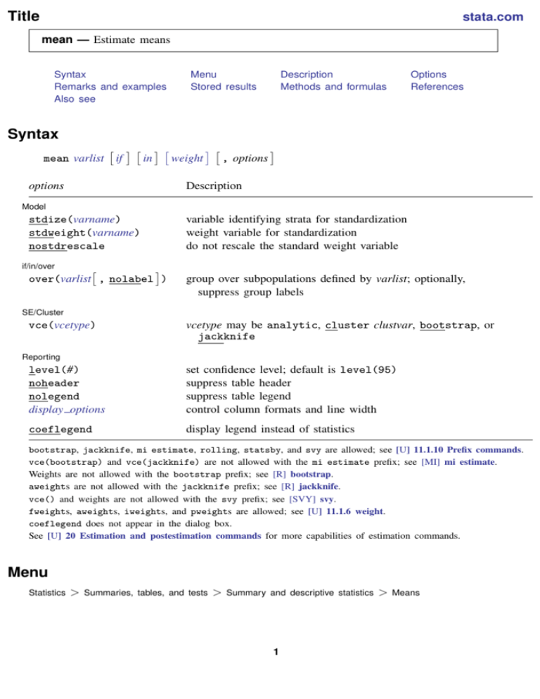
Title
stata.com
mean — Estimate means
Syntax
Remarks and examples
Also see
Menu
Stored results
Description
Methods and formulas
Options
References
Syntax
mean varlist if
in
weight
, options
Description
options
Model
stdize(varname)
stdweight(varname)
nostdrescale
variable identifying strata for standardization
weight variable for standardization
do not rescale the standard weight variable
if/in/over
over(varlist , nolabel )
group over subpopulations defined by varlist; optionally,
suppress group labels
SE/Cluster
vce(vcetype)
vcetype may be analytic, cluster clustvar, bootstrap, or
jackknife
Reporting
level(#)
noheader
nolegend
display options
set confidence level; default is level(95)
suppress table header
suppress table legend
control column formats and line width
coeflegend
display legend instead of statistics
bootstrap, jackknife, mi estimate, rolling, statsby, and svy are allowed; see [U] 11.1.10 Prefix commands.
vce(bootstrap) and vce(jackknife) are not allowed with the mi estimate prefix; see [MI] mi estimate.
Weights are not allowed with the bootstrap prefix; see [R] bootstrap.
aweights are not allowed with the jackknife prefix; see [R] jackknife.
vce() and weights are not allowed with the svy prefix; see [SVY] svy.
fweights, aweights, iweights, and pweights are allowed; see [U] 11.1.6 weight.
coeflegend does not appear in the dialog box.
See [U] 20 Estimation and postestimation commands for more capabilities of estimation commands.
Menu
Statistics
>
Summaries, tables, and tests
>
Summary and descriptive statistics
1
>
Means
2
mean — Estimate means
Description
mean produces estimates of means, along with standard errors.
Options
Model
stdize(varname) specifies that the point estimates be adjusted by direct standardization across the
strata identified by varname. This option requires the stdweight() option.
stdweight(varname) specifies the weight variable associated with the standard strata identified in
the stdize() option. The standardization weights must be constant within the standard strata.
nostdrescale prevents the standardization weights from being rescaled within the over() groups.
This option requires stdize() but is ignored if the over() option is not specified.
if/in/over
over(varlist , nolabel ) specifies that estimates be computed for multiple subpopulations, which
are identified by the different values of the variables in varlist.
When this option is supplied with one variable name, such as over(varname), the value labels of
varname are used to identify the subpopulations. If varname does not have labeled values (or there
are unlabeled values), the values themselves are used, provided that they are nonnegative integers.
Noninteger values, negative values, and labels that are not valid Stata names are substituted with
a default identifier.
When over() is supplied with multiple variable names, each subpopulation is assigned a unique
default identifier.
nolabel requests that value labels attached to the variables identifying the subpopulations be
ignored.
SE/Cluster
vce(vcetype) specifies the type of standard error reported, which includes types that are derived from
asymptotic theory (analytic), that allow for intragroup correlation (cluster clustvar), and that
use bootstrap or jackknife methods (bootstrap, jackknife); see [R] vce option.
vce(analytic), the default, uses the analytically derived variance estimator associated with the
sample mean.
Reporting
level(#); see [R] estimation options.
noheader prevents the table header from being displayed. This option implies nolegend.
nolegend prevents the table legend identifying the subpopulations from being displayed.
display options: cformat(% fmt) and nolstretch; see [R] estimation options.
The following option is available with mean but is not shown in the dialog box:
coeflegend; see [R] estimation options.
mean — Estimate means
Remarks and examples
3
stata.com
Example 1
Using the fuel data from example 3 of [R] ttest, we estimate the average mileage of the cars
without the fuel treatment (mpg1) and those with the fuel treatment (mpg2).
. use http://www.stata-press.com/data/r13/fuel
. mean mpg1 mpg2
Mean estimation
Number of obs
mpg1
mpg2
=
12
Mean
Std. Err.
[95% Conf. Interval]
21
22.75
.7881701
.9384465
19.26525
20.68449
22.73475
24.81551
Using these results, we can test the equality of the mileage between the two groups of cars.
. test mpg1 = mpg2
( 1) mpg1 - mpg2 = 0
F( 1,
11) =
Prob > F =
5.04
0.0463
Example 2
In example 1, the joint observations of mpg1 and mpg2 were used to estimate a covariance between
their means.
. matrix list e(V)
symmetric e(V)[2,2]
mpg1
mpg2
mpg1 .62121212
mpg2
.4469697 .88068182
If the data were organized this way out of convenience but the two variables represent independent
samples of cars (coincidentally of the same sample size), we should reshape the data and use the
over() option to ensure that the covariance between the means is zero.
. use http://www.stata-press.com/data/r13/fuel
. stack mpg1 mpg2, into(mpg) clear
. mean mpg, over(_stack)
Mean estimation
1: _stack = 1
2: _stack = 2
Number of obs
=
24
Over
Mean
Std. Err.
[95% Conf. Interval]
1
2
21
22.75
.7881701
.9384465
19.36955
20.80868
mpg
22.63045
24.69132
4
mean — Estimate means
. matrix list e(V)
symmetric e(V)[2,2]
mpg:
mpg:
1
2
mpg:1 .62121212
mpg:2
0 .88068182
Now we can test the equality of the mileage between the two independent groups of cars.
. test [mpg]1 = [mpg]2
( 1) [mpg]1 - [mpg]2 = 0
F( 1,
23) =
2.04
Prob > F =
0.1667
Example 3: standardized means
Suppose that we collected the blood pressure data from example 2 of [R] dstdize, and we wish to
obtain standardized high blood pressure rates for each city in 1990 and 1992, using, as the standard,
the age, sex, and race distribution of the four cities and two years combined. Our rate is really the
mean of a variable that indicates whether a sampled individual has high blood pressure. First, we
generate the strata and weight variables from our standard distribution, and then use mean to compute
the rates.
. use http://www.stata-press.com/data/r13/hbp, clear
. egen strata = group(age race sex) if inlist(year, 1990, 1992)
(675 missing values generated)
. by strata, sort: gen stdw = _N
. mean hbp, over(city year) stdize(strata) stdweight(stdw)
Mean estimation
N. of std strata =
24
Number of obs
=
455
Over: city year
_subpop_1: 1 1990
_subpop_2: 1 1992
_subpop_3: 2 1990
_subpop_4: 2 1992
_subpop_5: 3 1990
_subpop_6: 3 1992
_subpop_7: 5 1990
_subpop_8: 5 1992
Over
Mean
hbp
_subpop_1
_subpop_2
_subpop_3
_subpop_4
_subpop_5
_subpop_6
_subpop_7
_subpop_8
.058642
.0117647
.0488722
.014574
.1011211
.0810577
.0277778
.0548926
Std. Err.
.0296273
.0113187
.0238958
.007342
.0268566
.0227021
.0155121
0
[95% Conf. Interval]
.0004182
-.0104789
.0019121
.0001455
.0483425
.0364435
-.0027066
.
.1168657
.0340083
.0958322
.0290025
.1538998
.1256719
.0582622
.
The standard error of the high blood pressure rate estimate is missing for city 5 in 1992 because
there was only one individual with high blood pressure; that individual was the only person observed
in the stratum of white males 30–35 years old.
mean — Estimate means
5
By default, mean rescales the standard weights within the over() groups. In the following, we
use the nostdrescale option to prevent this, thus reproducing the results in [R] dstdize.
. mean hbp, over(city year) nolegend stdize(strata) stdweight(stdw)
> nostdrescale
Mean estimation
N. of std strata =
24
Number of obs
=
455
Over
Mean
hbp
_subpop_1
_subpop_2
_subpop_3
_subpop_4
_subpop_5
_subpop_6
_subpop_7
_subpop_8
.0073302
.0015432
.0078814
.0025077
.0155271
.0081308
.0039223
.0088735
Std. Err.
.0037034
.0014847
.0038536
.0012633
.0041238
.0022772
.0021904
0
[95% Conf. Interval]
.0000523
-.0013745
.0003084
.000025
.007423
.0036556
-.0003822
.
Video example
Descriptive statistics in Stata
Stored results
mean stores the following in e():
Scalars
e(N)
e(N over)
e(N stdize)
e(N clust)
e(k eq)
e(df r)
e(rank)
Macros
e(cmd)
e(cmdline)
e(varlist)
e(stdize)
e(stdweight)
e(wtype)
e(wexp)
e(title)
e(cluster)
e(over)
e(over labels)
e(over namelist)
e(vce)
e(vcetype)
e(properties)
e(estat cmd)
e(marginsnotok)
number of observations
number of subpopulations
number of standard strata
number of clusters
number of equations in e(b)
sample degrees of freedom
rank of e(V)
mean
command as typed
varlist
varname from stdize()
varname from stdweight()
weight type
weight expression
title in estimation output
name of cluster variable
varlist from over()
labels from over() variables
names from e(over labels)
vcetype specified in vce()
title used to label Std. Err.
b V
program used to implement estat
predictions disallowed by margins
.0146082
.004461
.0154544
.0049904
.0236312
.012606
.0082268
.
6
mean — Estimate means
Matrices
e(b)
e(V)
e( N)
e( N stdsum)
e( p stdize)
e(error)
Functions
e(sample)
vector of mean estimates
(co)variance estimates
vector of numbers of nonmissing observations
number of nonmissing observations within the standard strata
standardizing proportions
error code corresponding to e(b)
marks estimation sample
Methods and formulas
Methods and formulas are presented under the following headings:
The mean estimator
Survey data
The survey mean estimator
The standardized mean estimator
The poststratified mean estimator
The standardized poststratified mean estimator
Subpopulation estimation
The mean estimator
Let y be the variable on which we want to calculate the mean and yj an individual observation on
y , where j = 1, . . . , n and n is the sample size. Let wj be the weight, and if no weight is specified,
define wj = 1 for all j . For aweights, the wj are normalized to sum to n. See The survey mean
estimator for pweighted data.
Let W be the sum of the weights
W =
n
X
wj
j=1
The mean is defined as
y=
n
1 X
wj yj
W j=1
The default variance estimator for the mean is
n
Vb (y) =
X
1
wj (yj − y)2
W (W − 1) j=1
The standard error of the mean is the square root of the variance.
If x, xj , and x are similarly defined for another variable (observed jointly with y ), the covariance
estimator between x and y is
n
d
Cov(x,
y) =
X
1
wj (xj − x)(yj − y)
W (W − 1) j=1
mean — Estimate means
7
Survey data
See [SVY] variance estimation, [SVY] direct standardization, and [SVY] poststratification for
discussions that provide background information for the following formulas. The following formulas
are derived from the fact that the mean is a special case of the ratio estimator where the denominator
variable is one, xj = 1; see [R] ratio.
The survey mean estimator
Let Yj be a survey item for the j th individual in the population, where j = 1, . . . , M and M
is the size of the population. The associated population mean for the item of interest is Y = Y /M
where
M
X
Yj
Y =
j=1
Let yj be the survey item for the j th sampled individual from the population, where j = 1, . . . , m
and m is the number of observations in the sample.
c, where
The estimator for the mean is y = Yb /M
Yb =
m
X
wj yj
c=
M
and
m
X
j=1
wj
j=1
and wj is a sampling weight. The score variable for the mean estimator is
zj (y) =
cyj − Yb
yj − y
M
=
c
c2
M
M
The standardized mean estimator
Let Dg denote the set of sampled observations that belong to the g th standard stratum and define
IDg (j) to indicate if the j th observation is a member of the g th standard stratum; where g = 1, . . . ,
LD and LD is the number of standard strata. Also, let πg denote the fraction of the population that
belongs to the g th standard stratum, thus π1 + · · · + πLD = 1. πg is derived from the stdweight()
option.
The estimator for the standardized mean is
yD =
LD
X
πg
g=1
where
Ybg =
m
X
IDg (j) wj yj
Ybg
cg
M
and
j=1
cg =
M
m
X
j=1
The score variable for the standardized mean is
zj (y D ) =
LD
X
g=1
πg IDg (j)
cg yj − Ybg
M
cg2
M
IDg (j) wj
8
mean — Estimate means
The poststratified mean estimator
Let Pk denote the set of sampled observations that belong to poststratum k and define IPk (j)
to indicate if the j th observation is a member of poststratum k ; where k = 1, . . . , LP and LP is
the number of poststrata. Also let Mk denote the population size for poststratum k . Pk and Mk are
identified by specifying the poststrata() and postweight() options on svyset; see [SVY] svyset.
The estimator for the poststratified mean is
yP =
where
Yb P =
LP
X
Mk
ck
M
k=1
and
cP =
M
Yb P
Yb P
=
cP
M
M
LP
m
X
Mk X
Ybk =
k=1
LP
X
Mk
k=1
ck
M
LP
X
ck =
M
ck
M
IPk (j) wj yj
j=1
Mk = M
k=1
The score variable for the poststratified mean is
LP
Mk
zj (Yb P )
1 X
IPk (j)
zj (y ) =
=
ck
M
M
M
P
k=1
Ybk
yj −
ck
M
!
The standardized poststratified mean estimator
The estimator for the standardized poststratified mean is
y DP =
LD
X
YbgP
cgP
M
πg
g=1
where
YbgP =
Lp
X
Mk
k=1
and
cgP =
M
ck
M
Ybg,k =
k=1
Lp
X
Mk
k=1
Lp
m
X
Mk X
ck
M
cg,k =
M
ck
M
IDg (j)IPk (j) wj yj
j=1
Lp
m
X
Mk X
k=1
ck
M
IDg (j)IPk (j) wj
j=1
The score variable for the standardized poststratified mean is
zj (y DP ) =
LD
X
g=1
where
zj (YbgP )
=
LP
X
k=1
and
cP )
zj ( M
g
=
πg
cgP zj (YbgP ) − YbgP zj (M
cgP )
M
cP )2
(M
Mk
IPk (j)
ck
M
LP
X
k=1
g
(
Mk
IPk (j)
ck
M
Ybg,k
IDg (j)yj −
ck
M
(
cg,k
M
IDg (j) −
ck
M
)
)
mean — Estimate means
9
Subpopulation estimation
Let S denote the set of sampled observations that belong to the subpopulation of interest, and
define IS (j) to indicate if the j th observation falls within the subpopulation.
cS , where
The estimator for the subpopulation mean is y S = Yb S /M
Yb S =
m
X
IS (j) wj yj
cS =
M
and
j=1
m
X
IS (j) wj
j=1
Its score variable is
zj (y S ) = IS (j)
cS yj − Yb S
yj − y S
M
= IS (j)
cS )2
cS
(M
M
The estimator for the standardized subpopulation mean is
y DS =
LD
X
πg
g=1
where
YbgS =
m
X
IDg (j)IS (j) wj yj
YbgS
cgS
M
cgS =
M
and
j=1
m
X
IDg (j)IS (j) wj
j=1
Its score variable is
zj (y DS ) =
LD
X
πg IDg (j)IS (j)
g=1
cgS yj − YbgS
M
cgS )2
(M
The estimator for the poststratified subpopulation mean is
yP S =
where
Yb P S =
LP
X
Mk
k=1
and
cP S =
M
ck
M
YbkS =
k=1
LP
m
X
Mk X
k=1
LP
X
Mk
ck
M
Yb P S
cP S
M
ckS =
M
ck
M
IPk (j)IS (j) wj yj
j=1
LP
m
X
Mk X
k=1
ck
M
IPk (j)IS (j) wj
j=1
Its score variable is
zj (y P S ) =
where
bPS
zj ( Y
)=
cP S zj (Yb P S ) − Yb P S zj (M
cP S )
M
cP S )2
(M
LP
X
k=1
Mk
IPk (j)
ck
M
(
Yb S
IS (j) yj − k
ck
M
)
10
mean — Estimate means
and
cP S ) =
zj (M
LP
X
k=1
Mk
IPk (j)
ck
M
(
cS
M
IS (j) − k
ck
M
)
The estimator for the standardized poststratified subpopulation mean is
y DP S =
LD
X
πg
g=1
where
YbgP S =
Lp
X
Mk
k=1
and
cgP S =
M
ck
M
S
Ybg,k
=
k=1
Lp
m
X
Mk X
k=1
Lp
X
Mk
ck
M
YbgP S
cgP S
M
S
cg,k
M
=
ck
M
IDg (j)IPk (j)IS (j) wj yj
j=1
Lp
m
X
Mk X
k=1
ck
M
IDg (j)IPk (j)IS (j) wj
j=1
Its score variable is
zj (y DP S ) =
LD
X
g=1
where
zj (YbgP S )
=
LP
X
k=1
and
cgP S ) =
zj (M
πg
cP S zj (Yb P S ) − Yb P S zj (M
cP S )
M
g
g
g
g
cgP S )2
(M
Mk
IPk (j)
ck
M
LP
X
k=1
(
Mk
IPk (j)
ck
M
S
Ybg,k
IDg (j)IS (j) yj −
ck
M
(
cS
M
g,k
IDg (j)IS (j) −
ck
M
)
)
References
Bakker, A. 2003. The early history of average values and implications for education. Journal of Statistics Education
11(1). http://www.amstat.org/publications/jse/v11n1/bakker.html.
Cochran, W. G. 1977. Sampling Techniques. 3rd ed. New York: Wiley.
Stuart, A., and J. K. Ord. 1994. Kendall’s Advanced Theory of Statistics: Distribution Theory, Vol I. 6th ed. London:
Arnold.
mean — Estimate means
Also see
[R] mean postestimation — Postestimation tools for mean
[R] ameans — Arithmetic, geometric, and harmonic means
[R] proportion — Estimate proportions
[R] ratio — Estimate ratios
[R] summarize — Summary statistics
[R] total — Estimate totals
[MI] estimation — Estimation commands for use with mi estimate
[SVY] direct standardization — Direct standardization of means, proportions, and ratios
[SVY] poststratification — Poststratification for survey data
[SVY] subpopulation estimation — Subpopulation estimation for survey data
[SVY] svy estimation — Estimation commands for survey data
[SVY] variance estimation — Variance estimation for survey data
[U] 20 Estimation and postestimation commands
11