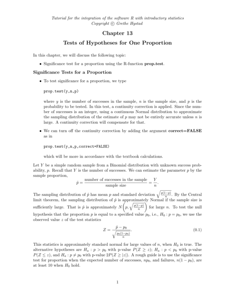
Tutorial for the integration of the software R with introductory statistics
c Grethe Hystad
Copyright Chapter 13
Tests of Hypotheses for One Proportion
In this chapter, we will discuss the following topic:
• Significance test for a proportion using the R-function prop.test.
Significance Tests for a Proportion
• To test significance for a proportion, we type
prop.test(y,n,p)
where y is the number of successes in the sample, n is the sample size, and p is the
probability to be tested. In this test, a continuity correction is applied. Since the number of successes is an integer, using a continuous Normal distribution to approximate
the sampling distribution of the estimate of p may not be entirely accurate unless n is
large. A continuity correction will compensate for that.
• We can turn off the continuity correction by adding the argument correct=FALSE
as in
prop.test(y,n,p,correct=FALSE)
which will be more in accordance with the textbook calculations.
Let Y be a simple random sample from a Binomial distribution with unknown success probability, p. Recall that Y is the number of successes. We can estimate the parameter p by the
sample proportion,
number of successes in the sample
Y
p̂ =
= .
sample size
n
q
The sampling distribution of p̂ has mean p and standard deviation p(1−p)
n . By the Central
limit theorem, the sampling distribution of p̂ is approximately
Normal
if the sample size is
q
p(1−p)
n
sufficiently large. That is p̂ is approximately N p,
for large n. To test the null
hypothesis that the proportion p is equal to a specified value p0 , i.e., H0 : p = p0 , we use the
observed value z of the test statistics
p̂ − p0
Z=q
.
(0.1)
p0 (1−p0 )
n
This statistics is approximately standard normal for large values of n, when H0 is true. The
alternative hypotheses are Ha : p > p0 with p-value P (Z ≥ z); Ha : p < p0 with p-value
P (Z ≤ z), and Ha : p 6= p0 with p-value 2P (Z ≥ |z|). A rough guide is to use the significance
test for proportion when the expected number of successes, np0 , and failures, n(1 − p0 ), are
at least 10 when H0 hold.
1
An approximate 100(1 − α)% confidence interval for p is
r
p̂(1 − p̂)
p̂ ± z ∗
,
n
(0.2)
where the critical value z ∗ is chosen such that the area under the normal density curve
between −z ∗ and z ∗ is (1 − α). In order to use this confidence interval, the numbers of
successes and failures should both be at least 15 [3].
Problem. The Trial Urban District Assessment (TUDA) is a study sponsored by the government of student achievement in large urban school districts. The math test-score is on a
scale from 0 to 500. A ”basic” math level is a score of 262, a ”proficient” level is a score of
299, and a ”advanced” level is a score of 333. In 2011, between 1,000 and 2,700 fourth- and
eighth-graders from public schools in 21 urban districts participated in the NAEP TUDA in
mathematics [1].
In 2011, 792 of a random sample of 1200 eighth-graders in San Diego scored above the Basic
level in mathematics. In large public city, 63% scored above the Basic level in mathematics
[2]. (The study reports the proportions).
(A) Is the proportion of eighth-graders who scored above the Basic level in mathematics in
San Diego significantly larger than 0.63 at the 5% level?
(B) Calculate a 99% confidence interval for the proportion of eight-graders who scored above
the Basic level in mathematics in San Diego.
Solution to part (a). Let p be the proportion of eighth-graders in San Diego that scored
above the Basic level in mathematics. We wish to test the null hypothesis that the proportion
p is equal to 0.63 against the alternative hypothesis that p is greater than 0.63. That is, we
wish to test
H0 : p = 0.63 against Ha : p > 0.63.
We obtain:
> prop.test(792,1200,0.63,alternative=c("greater"),correct=FALSE)
1-sample proportions test without continuity correction
data: 792 out of 1200, null probability 0.63
X-squared = 4.6332, df = 1, p-value = 0.01568
alternative hypothesis: true p is greater than 0.63
95 percent confidence interval:
0.6371695 1.0000000
sample estimates:
p
0.66
Since the p-value is 0.01568 < 0.05, we reject the null hypothesis at the 5% level. Thus, we
have strong evidence that the proportion of eighth-graders who scored above the Basic level
in mathematics in San Diego is greater than 0.63.
2
Solution to part (b). We first calculate the confidence interval using the textbook formula
in (0.2): We have 0.99 + (1 − 0.99)/2 = 0.995, so we wish to find z ∗ such that P (Z ≤ z ∗ ) =
0.995. We obtain:
> phat=792/1200
> z=qnorm(0.995)
> conf=c(phat-z*sqrt((phat*(1-phat))/1200),phat+z*sqrt((phat*(1-phat))/1200))
> conf
[1] 0.6247761 0.6952239
The 99% confidence interval for the proportion of eighth-graders who scored above the Basic
level in mathematics in San Diego is (0.625, 0.695). Thus, we are 99% confident that the
percent of eighth-graders who scored above the Basic level in mathematics in San Diego is
between 62.5% and 69.5%.
If we do this calculation in R, we obtain:
> prop.test(792,1200, conf.level=0.99,correct=FALSE)
1-sample proportions test without continuity correction
data: 792 out of 1200, null probability 0.5
X-squared = 122.88, df = 1, p-value < 2.2e-16
alternative hypothesis: true p is not equal to 0.5
99 percent confidence interval:
0.6239822 0.6942582
sample estimates:
p
0.66
R obtains a slightly different result due to the fact that R uses a different method for
calculating confidence intervals for one proportion.
Explanation. The code can be explained as follows:
• The prop.test in R computes a chi-squared statistic, X -squared, (see chapter 22 for
the definition of chi-squared statistics).
This test is equivalent to the z-test when you
√
take its square root, that is, z = 4.6332 = 2.152487.
• We added the argument correct=FALSE to turn off the continuity correction such
that the z statistics is equivalent to the textbook formula in (0.1).
References
[1]
National Assessment of Educational Progress, National Center for Education Statistics,
National Assessment Governing Board, Institute of Education Sciences, U.S. Department
of Education at http://nationsreportcard.gov/tuda.asp
[2]
National Center for Education Statistics, The Nation’s Report Card, Mathematics 2011,
Trial Urban District Assessment, Results at grades 4 and 8, Institute of Education Sciences, U.S. Department of Education, NCES 2012-452.
3
[3]
D. S. Moore, W. I. Notz, M. A. Fligner, R. Scoot Linder. The Basic Practice of Statistics.
W. F. Freeman and Company, New York, 2013.
00
4