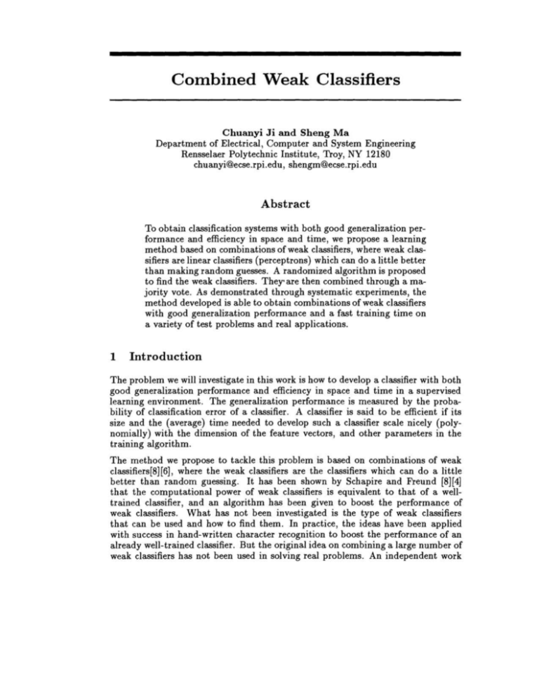
Combined Weak Classifiers
Chuanyi Ji and Sheng Ma
Department of Electrical, Computer and System Engineering
Rensselaer Polytechnic Institute, Troy, NY 12180
chuanyi@ecse.rpi.edu, shengm@ecse.rpi.edu
Abstract
To obtain classification systems with both good generalization performance and efficiency in space and time, we propose a learning
method based on combinations of weak classifiers, where weak classifiers are linear classifiers (perceptrons) which can do a little better
than making random guesses. A randomized algorithm is proposed
to find the weak classifiers. They· are then combined through a majority vote. As demonstrated through systematic experiments, the
method developed is able to obtain combinations of weak classifiers
with good generalization performance and a fast training time on
a variety of test problems and real applications.
1
Introduction
The problem we will investigate in this work is how to develop a classifier with both
good generalization performance and efficiency in space and time in a supervised
learning environment. The generalization performance is measured by the probability of classification error of a classifier. A classifier is said to be efficient if its
size and the (average) time needed to develop such a classifier scale nicely (polynomiaUy) with the dimension of the feature vectors, and other parameters in the
training algorithm.
The method we propose to tackle this problem is based on combinations of weak
classifiers [8][6] , where the weak classifiers are the classifiers which can do a little
better than random guessing . It has been shown by Schapire and Freund [8][4]
that the computational power of weak classifiers is equivalent to that of a welltrained classifier, and an algorithm has been given to boost the performance of
weak classifiers. What has not been investigated is the type of weak classifiers
that can be used and how to find them. In practice, the ideas have been applied
with success in hand-written character recognition to boost the performance of an
already well-trained classifier. But the original idea on combining a large number of
weak classifiers has not been used in solving real problems. An independent work
Combinations of Weak Classifiers
495
by Kleinberg[6] suggests that in addition to a good generalization performance,
combinations of weak classifiers also provide advantages in computation time, since
weak classifiers are computationally easier to obtain than well-trained classifiers.
However, since the proposed method is based on an assumption which is difficult
to realize, discrepancies have been found between the theory and the experimental
results[7]. The recent work by Breiman[1][2] also suggests that combinations of
classifiers can be computationally efficient, especially when used to learn large data
sets.
The focus of this work is to investigate the following problems: (1) how to find
weak classifiers, (2) what are the performance and efficiency of combinations of
weak classifiers, and (3) what are the advantages of using combined weak classifiers
compared with other pattern classification methods?
We will develop a randomized algorithm to obtain weak classifiers. We will then
provide simulation results on both synthetic real problems to show capabilities and
efficiency of combined weak classifiers. The extended version of this work with some
of the theoretical analysis can be found in [5].
2
Weak Classifiers
In the present work, we choose linear classifiers (perceptrons) as weak classifiers.
~ be the required generalization error of a classifier, where v 2: 2, is called
Let
the weakness factor which is used to characterize the strength of a classifier. The
larger the v, the weaker the weak classifier. A set of weak classifiers are combined
through a simple majority vote.
t-
3
Algorithm
Our algorithm for combinations of weak classifiers consists of two steps: (1) generating individual weak classifiers through a simple randomized algorithm; and (2)
combining a collection of weak classifiers through a simple majority vote.
Three parameters need to be chosen a priori for the algorithm: a weakness factor v,
a number (J (~ ~ (J < 1) which will be used as a threshold to partition the training
set, and the number of weak classifiers 2£ + 1 to be generated, where £ is a positive
integer.
3.1
Partitioning the Training Set
The method we use to partition a training set is motivated by what given in [4].
Suppose a combined classifier consists of K (K ~ 1) weak classifiers already. In
order to generate a (new) weak classifier, the entire training set of N training
samples is partitioned into two subsets: a set of Ml samples which contain all
the misclassified samples and a small fraction of samples correctly-classified by the
existing combined classifier; and the remaining N - Ml training samples. The set of
Ml samples are called "cares", since they will be used to select a new weak classifier,
while the rest of the samples are the "don't-cares".
The threshold (J is used to determine which samples should be assigned as cares.
For instance, for the n-th training sample (1 ~ n ~ N), the performance index
a( n) is recorded, where a( n) is the fraction of the weak classifiers in the existing
combined classifier which classify the n-th sample correctly. If a(n) < (J, this sample
is assigned to the cares. Otherwise, it is a don't-care. This is done for all N samples.
496
C. Ji and S. Ma
Through partitioning a training set in this way, a newly-generated weak classifier
is forced to learn the samples which have not been learned by the existing weak
classifiers. In the meantime, a properly-chosen () can ensure that enough samples
are used to obtain each weak classifier.
3.2
Random Sampling
To achieve a fast training time, we obtain a weak classifier by randomly sampling
the classifier-space of all possible linear classifiers.
Assume that a feature vector x E Rd is distributed over a compact region D. The
direction of a hyperplane characterized by a linear classifier with a weight vector,
is first generated by randomly selecting the elements of the weight vector based
on a uniform distribution over (-1 , l)d . Then the threshold of the hyperplane
is determined by randomly picking an xED , and letting the hyperplane pass
through x . This will generate random hyperplanes which pass through the region
D, and whose directions are randomly distributed in all directions. Such a randomly
selected classifier will then be tested on all the cares. If it misclassifies a fraction of
cares no more than
~
€ (€ > 0 and small), the classifier is kept and will be
used in the combination. Otherwise, it is discarded . This process is repeated until
a weak classifier is finally obtained.
k- -
A newly-generated weak classifier is then combined with the existing ones through
a simple majority vote. The entire training set will then be tested on the combined
classifier to result in a new set of cares, and don't-cares. The whole process will
be repeated until the total number 2L + 1 of weak classifiers are generated. The
algorithm can be easily extended to multiple classes. Details can be found in [5] .
4
Experimental Results
Extensive simulations have been carried out on both synthetic and real problems
using our algorithm. One synthetic problem is chosen to test the efficiency of
our method. Real applications from standard data bases are selected to compare
the generalization performance of combinations of weak classifiers (CW) with that
of other methods such as K-Nearest-Neighbor classifiers (K-NN)l, artificial neural
networks (ANN), combinations of neural networks (CNN), and stochastic discriminations (SD).
4.1
A Synthetic Problem: Two Overlapping Gaussians
To test the scaling properties of combinations of weak classifiers, a non-linearly
separable problem is chosen from a standard database called ELENA 2. The problem is a two-class classification problem, where the distributions of samples in both
classes are multi-variate Gaussians with the same mean but different variances for
each independent variable. There is a considerable amount of overlap between the
samples in two classes, and the problem is non-linearly separable. The average generalization error and the standard deviations are given in Figure 1 for our algorithm
based on 20 runs, and for other classifiers. The Bayes error is also given to show
the theoretical limit. The results show that the performance of kNN degrades very
quickly. The performance of ANN is better than that of kNN but still deviates more
and more from the Bayes error as d gets large. The combination of weak classifiers
1 The
2
best result of different k is reported.
I pu b I neural-nets I ELEN AIdatabases IBenchmarks. ps. Z
on ft p.dice. ucl. ac. be
497
Combinations of Weak Classifiers
" I.,
- "- k-NN
-_ ANN
10
-0-
-
.....
cw
IV_
Figure 1: Performance versus the dimension of the feature vectors
Algorithms
Combined Weak Classifiers
k Nearest Neighbor
Neural Networks
Combined Neural Networks
Card1
(%) Error /er
11.3/ 0.85
15.67
13.64/ 0.85
13.02/0.33
Diabetes1
(%) Error / er
22.70/ 0.70
25.8
23.52/ 0.72
22.79/0.57
Gene1
(%1 Error/ er
11.80/0.52
22.87
13.47/0.44
12.08/0.23
Table 1: Performance on Card1, Diabetes1 and Gene1. er: standard deviation
continues to follow the trend of the Bayes error.
4.2
Proben1 Data Sets
Three data sets, Card1, Diabetes1 and Gene1 were selected to test our algorithm
from Proben1 databases which contain data sets from real applications3 .
Card1 data set is for a problem on determining whether a credit-card application
from a customer can be approved based on information given in 51-dimensional
feature vectors. 345 out of 690 examples are used for training and the rest for
testing. Diabetes1 data set is for determining whether diabetes is present based
on 8-dimensional input patterns. 384 examples are used for training and the same
number of samples for testing. Gene1 data set is for deciding whether a DNA
sequence is from a donor, an acceptor or neither from 120 dimensional binary feature
vectors. 1588 samples out of total of 3175 were used for training, and the rest for
testing.
The average generalization error as well as the standard deviations are reported in
Table 1. The results from combinations of weak classifiers are based on 25 runs.
The results of neural networks and combinations of well-trained neural networks are
from the database . As demonstrated by the results, combinations of weak classifiers
have been able to achieve the generalization performance comparable to or better
than that of combinations of well-trained neural networks.
4.3
Hand-written Digit Recognition
Hand-written digit recognition is chosen to test our algorithm, since one of
the previously developed method on combinations of weak classifiers (stochastic
discrimination[6]) was applied to this problem. For the purpose of comparison, the
3 Available
by
anonymous
ftp
/ pub/papers/techreports/1994/1994-21. ps.z.
from
ftp.ira.uka.de,
as
498
C. Ji and S. Ma
Algorithms
Combined Weak Classifiers
k Nearest Neighbor
Neural Networks
Stochastic Discriminations
(%) Error/O'
4.23/ 0.1
4.84
5.33
3.92
Table 2: Performance on handwritten digit recognition.
Parameters
1/2 + l/v
e
2L+1
A verage Tries
Gaussians
0.51
0.51
2000
2
Card1
0.51
0.51
1000
3
Diabetes1
0.51
0.54
1000
7
Gene1
0.55
0.54
4000
4
Digits
0.54
0.53
20000
2
Table 3: Parameters used in our experiments.
same set of data as used in [6](from the NIST data base) is utilized to train and
to test our algorithm. The data set contains 10000 digits written by different people. Each digit is represented by 16 by 16 black and white pixels. The first 4997
digits are used to form a training set, and the rest are for testing. Performance
of our algorithm, k-NN, neural networks, and stochastic discriminations are given
in Table 2. The results for our methods are based on 5 runs, while the results
for the other methods are from [6]. The results show that the performance of our
algorithm is slightly worse (by 0.3%) than that of stochastic discriminations, which
uses a different method for multi-class classification [6] .
4.4
Effects of The Weakness Factor
Experiments are done to test the effects of v on the problem of two 8-dimensional
overlapping Gaussians. The performance and the average training time (CPUtime on Sun Spac-10) of combined weak classifiers based on 10 runs are given for
different v's in Figures 2 and 3, respectively. The results indicate as v increases
an individual weak classifier is obtained more quickly, but more weak classifiers are
needed to achieve good performance. When a proper v is chosen, a nice scaling
property can be observed in training time.
A record of the parameters used in all the experiments on real applications are
provided in Table 3. The average tries, which are the average number of times
needed to sample the classifier space to obtain an acceptable weak classifier, are
also given in the table to characterize the training time for these problems.
4.5
Training Time
To compare learning time with off-line BackPropagation (BP), feedforward two layer
neural network with 10 sigmoidal hidden units are trained by gradient-descent to
learn the problem on the two 8-dimensional overlapping Gaussians. 2500 training
samples are used. The performance versus CPU time 4 are plotted for both our
algorithm and BP in Figure 4. For our algorithm, 2000 weak classifiers are combined. For BP, 1000 epoches are used. The figure shows that our algorithm is much
faster than the BP algorithm. Moreover, when several well-trained neural networks
are combined to achieve a better performance, the cost on training time will be
4Both algorithms are run on a Sun Sparc-lO sun workstation
499
Combinations of Weak Classifiers
'°0
200
400
too
100
1000 1200 1400
NuntMI'oII . . . . ~
,'00
1100
2000
Figure 2: Performance versus the number of weak classifiers for different
I'
~
~
u
-0-
-x-
•
1/.
nu :
1/.
1AwaO 005
lJnu-o.Ol0
-·- · 1~O'5
,
-+- : lA'1u-002O
-
: lhN-0025
. .'
,
_
_
_
_
_~~::::
_ : :::::
_
_
_m "::;~~=1;:~-~:~~~~~oIIw.-a...r
...
Figure 3: Training time versus the number of weak classifiers for different
1/.
even higher. Therefore, compared to combinations of well-trained neural networks,
combining weak classifiers is computationally much cheaper.
5
Discussions
From the experimental results, we observe that the performance of the combined
weak classifiers is comparable or even better than combinations of well- trained classifiers, and out-performs individual neural network classifiers and k-Nearest Neighbor classifiers. In the meantime whereas the k-nearest neighbor classifiers suffer
from the curse of dimensionality, a nice scaling property in terms of the dimension of feature vectors has been observed for combined weak classifiers. Another
.
.
35
,,
,,
;
-
TranngcurteollBP
T_CV't'eollBP
T,......cuwolCW
- r_cwy.otcw
v_
I
IS
10
l --_
-1- -
-----..
.............. --t-___ ,
-
-
-
_
I- - _ _ __ t ____ _
I
Figure 4: Performance versus CPU time
500
C. Ii and S. Ma
important observation obtained from the experiments is that the weakness factor
directly impacts the size of a combined classifier and the training time. Therefore,
the choice of the weakness factor is important to obtain efficient combined weak
classifiers. It has been shown in our theoretical analysis on learning an underlying
perceptron [5] that v should be at least large as O( dlnd) to obtain a polynomial
training time, and the price paid to accomplish this is a space-complexity which is
polynomial in d as well. This cost can be observed from our experimental results
for the need of a large number of weak classifiers.
Acknowledgement
Specials thanks are due to Tin Kan Ho for providing NIST data, related references and helpful discussions. Support from the National Science Foundation (ECS9312594 and (CAREER) IRI-9502518) is gratefully acknowledged.
References
[1] L. Breiman, "Bias, Variance and Arcing Classifiers," Technical Report, TR460, Department of Statistics, University of California, Berkeley, April, 1996.
[2] 1. Breiman, "Pasting, Bites Together for Prediction in Large Data sets and
On-Line," ftp.stat .berkeley.edu/users/breiman, 1996.
[3] H. Drucker, R . Schapire and P. Simard, "Improving Performance in Neural
Networks Using a Boosting Algorithm," Neural Information Processing Symposium, 42-49, 1993.
[4] Y .
Freund
and
R.
Schapire,
"A
Decision-Theoretic Generalization of On-Line Learning and An Application
to Boosting," http://www.research.att.com/orgs/ssr/people/yoav or schapire.
[5] C. Ji and S. Ma, "Combinations of Weak Classifiers," IEEE Trans . Neural
Networks, Special Issue on Neural Networks and Pattern Recognition, vol. 8,
32-42, Jan., 1997.
[6] E .M. Kleinberg, "Stochastic Discrimination," Annals of Mathematics and Artificial Intelligence , voU , 207-239, 1990.
[7] E.M. Kleinberg and T. Ho, "Pattern Recognition by Stochastic Modeling,"
Proceedings of the Third International Workshop on Frontiers in Handwriting
Recognition, 175-183, Buffalo, May 1993.
[8] R.E. Schapire, "The Strength of Weak Learnability," Machine Learning, vol.
5, 197-227, 1990.