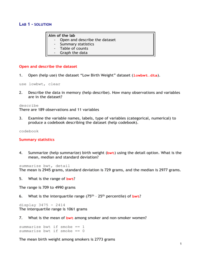
LAB 1 - SOLUTION
Aim of the lab
- Open and describe the dataset
- Summary statistics
- Table of counts
- Graph the data
Open and describe the dataset
1.
Open (help use) the dataset “Low Birth Weight” dataset (lowbwt.dta).
use lowbwt, clear
2.
Describe the data in memory (help describe). How many observations and variables
are in the dataset?
describe
There are 189 observations and 11 variables
3.
Examine the variable names, labels, type of variables (categorical, numerical) to
produce a codebook describing the dataset (help codebook).
codebook
Summary statistics
4.
Summarize (help summarize) birth weight (bwt) using the detail option. What is the
mean, median and standard deviation?
summarize bwt, detail
The mean is 2945 grams, standard deviation is 729 grams, and the median is 2977 grams.
5.
What is the range of bwt?
The range is 709 to 4990 grams
6.
What is the interquartile range (75th – 25th percentile) of bwt?
display 3475 - 2414
The interquartile range is 1061 grams
7.
What is the mean of bwt among smoker and non-smoker women?
summarize bwt if smoke == 1
summarize bwt if smoke == 0
The mean birth weight among smokers is 2773 grams
1
The mean birth weight among non-smokers is 3055 grams
Tables of frequencies
8.
Tabulate the binary outcome variable low (help tabulate). What is the proportion
of having a low birth weight in the sample?
tabulate low
The proportion of women having a low birth weight is 31.2%
9.
What is the proportion of women with history of hypertension?
tabulate ht
The proportion of women with history of hypertension 6.35%
10. What is the proportion of having a low birth weight among women with and without
history of hypertension (ht)?
tabulate low if ht == 1
tabulate low if ht == 0
The proportion of women having history of hypertension is 58%
The proportion of women having no history of hypertension is 29%
Graphs
11. Graph the distribution (using a histogram and a box-plot) of the continuous
outcome variable bwt. Interpret the graphs (help histogram, help graph box).
histogram bwt
graph box bwt
12. Create a horizontal box plot of the variable bwt by smoke status. What is the
difference in the distribution of bwt in the two groups?
graph hbox bwt , over(smoke)
Women who smoked during pregnancy were more likely to have a lower birth weight.
Normal distribution
13. Suppose that X is a random variable that represents the height of women ages 3075 in Sweden. Assume that X is normally distributed with a mean of 166 cm and a
standard deviation of 6 cm. What is the probability that a randomly selected
woman is less than 160 cm tall?
P(X < 60) = P[(X-)/ < (160 – 166)/6] = P(Z < -1) = 0.16
2
. di normal( -1 )
.15865525
Calculating Normal Probabilities with Stata
Like binomial probabilities, Stata can be used to calculate probabilities
associated with the standard normal distribution using the normal command.
To calculate the probability that a standard normal random variable Z is less
than some value k (i.e. P(Z<k), type
display normal(k)
If you want the probability that Z is greater than some value k (i.e. P(Z>k)),
then make use of the fact that P(Z<k)+ P(Z>k)=1 and use the command
display 1-normal(k)
If you have a random variable, X, that follows an arbitrary normal distribution
with mean  and standard deviation , you must first transform X into a
standard normal random variable Z before using the normal command.
To find the value Z of the standard normal distribution that cuts off an area of p
in the left tail of the standard normal curve use
display invnormal(p)
14. What is the probability that a randomly selected woman is greater than 175 cm tall?
P(X > 175) = P[(X-)/ > (175 – 166)/6] = 1- P(Z < (175 – 166)/6 ) = 0.07
. display 1- normal( (175 - 166)/6
.0668072
)
15. What is the probability that a randomly selected woman is between 160 and 170 cm
tall?
P(160 < X < 170) = P[(160-166)/6 <(X-)/ < (170 – 166)/6] = 0.59
. display normal( (170 - 166)/6
.58885221
) - normal( (160-166)/6 )
3
16. Among females in the United States between 18 and 74 years of age, diastolic blood
pressure is normally distributed with mean 77 mmHg and standard deviation 11.6
mmHg. What is the probability that a randomly selected woman has a diastolic
blood pressure less than 60 mmHg?
P(X<60) = P(Z< (60-77)/11.6) = .0713
. display normal((60-77)/11.6)
.07138993
17. What is the probability that she has a diastolic blood pressure greater than 90
mmHg?
P(X>90) = P(Z>(90-77)/11.6) = 0.13
. di 1-normal( (90-77)/11.6)
.13120999
18. What is the probability that she has a diastolic blood pressure between 60 and 90
mmHg?
P(60 < X < 90) = P[(60-77)/11.6 <(X-)/ < (90 – 77)/11.6] = 0.797
. display normal((90-77)/11.6 ) - normal((60 - 77)/11.6)
.79740008
4