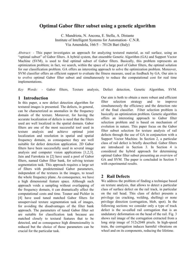
Optimal Gabor filter subset using a genetic algorithm
C. Mandriota, N. Ancona, E. Stella, A. Distante
Institute of Intelligent Systems for Automation– C.N.R.
Via Amendola, 166/5 – 70126 Bari (Italy)
Abstract: - This paper investigates an approach for analyzing textured material, as rail surface, using an
“optimal subset” of Gabor filters. A hybrid system, that ensemble Genetic Algorithm (GA) and Support Vector
Machine (SVM), is used to find optimal subset of Gabor filters. Basically, this problem represents an
optimization problem; in fact, we search, within the space of a large pool of Gabor filters, the optimal solution
for our classification problem. GA offers an interesting approach to solve the optimization problem. Moreover,
SVM classifier offers an efficient support to evaluate the fitness measure, used as feedback by GA. Our aim is
to evolve optimal Gabor filter subset and simultaneously to reduce the computational cost for real time
implementations.
Key
Words:
-
Gabor
filters,
Texture
analysis,
1 Introduction
In this paper, a new defect detection algorithm for
textured images is presented. The defects, in general,
can be characterized as anomalies in the frequency
domain of the texture. Moreover, for having the
accurate localization of defects is need that the filters
used are well localized in the spatial domain. Gabor
filters are one of the most successful tool used in
texture analysis and achieve optimal joint
localization and resolution in spatial and spatial
frequency domain, as consequence they are well
suitable for defect detection application. 2D Gabor
filters have been successfully used in several image
analysis and computer vision applications [1,2,3].
Jain and Farroknia in [2] have used a pool of Gabor
filters, named Gabor filter bank, for solving texture
segmentation task. This approach requires a large set
of filters with predetermined Gabor parameters,
independent of the textures in the images, to tessel
the whole frequency plane. As consequence, we have
a high dimensional feature space. Although such
approach voids a sampling without overlapping of
the frequency domain, it can dramatically affect the
computational costs and time. Teuner and Pichler in
[4] have used tuned matched Gabor filters for
unsupervised texture segmentation task of images,
for avoiding the disadvantages of the filter bank
approach. The parameters of tuned Gabor filter set
are suitable for classification task because are
matched closely to textural features that to be
detected, and as consequence high dimensionality is
reduced but the choice of those parameters can be
crucial for the particular task.
Defect
detection,
Genetic
Algorithm,
SVM.
Our aim is both to obtain a more robust and efficient
filter selection strategy and to improve
simultaneously the efficiency and the detection rate
of the final classifier. Filter selection problem is
basically an optimization problem. Genetic algorithm
offers an interesting approach to Gabor filter
selection problem and is based on mechanism of
evolution in nature. This paper focus on the Gabor
filter subset selection for texture analysis of rail
defects through the use of GA in conjunction with a
Support Vector Machine. In Section 2, a particular
class of rail defect is briefly described. Gabor filters
are introduced in Section 3. In Section 4 is
considered the hybrid approach for determining
optimal Gabor filter subset presenting an overview of
GA and SVM. The paper is concluded in Section 5
with experimental results.
2 Rail Defects
We address the problem of finding a technique based
on texture analysis, that allows to detect a particular
class of surface defect on the rail track, in particular
on the rail head. This class of defect presents a
privilege (as cracking, welding, shelling) or none
privilege direction (corrugation, blob, spot). In the
following sections we consider only a type of track
defect is the so-called rail corrugation that is an
undulatory deformation on the head of the rail. Fig. 3
shows rail image of the corrugation extracted from a
long strip image of 512x2048 pixels. In high-speed
train, the corrugation induces harmful vibrations on
wheel and on its components, reducing the lifetime.
and are depicted in Fig. 1. Next, for each filtered
image is evaluated the feature image as magnitude
.
3 Gabor Filters
The 2D Gabor functions are complex functions given
by the following expression  j   1  :
h
σ , , F
0
x  g1 ,2 , (x)  exp 2jF0x1' 
with  = (1, 2), where x’ is rotated coordinate of x
( x1' , x2'   x1 cos  x2 sin  ,x1 sin   x2 cos  ).
g1, 2,  represents a 2D Gaussian function with
standard deviations 1, 2 given by following
expression:
g 1 , 2 , x 
F0=
f   f 
0 2
1
0 2
2
 1  x 2 x 2 
1
 exp   12  22 
212
 2  1 2 
Fig. 1: Frequency (B) and half peak radial ()
bandwidths.
(1)
 f 20 

0 
 f1 
and  = tg–1 
are the
frequency and orientation of sinusoidal plane. In the
hypothesis that = , that is the modulating Gaussian
has the same orientation of the complex sine grating,
the Gabor function is always elongated in the
direction of the vector f0. The Fourier transform of a
2D Gabor function, as in equation (1), is given by the
following expression:
H ,,F0 (f1 , f 2 )  4 2 exp(2 2 (12 (f1'  F 0 ) 2   22 (f 2' ) 2 )) (2)
 
where f1' , f 2'  f1 cos  f 2 sin ,f1 sin   f 2 cos .. Note that,
the Fourier transform of a 2D Gabor function is a 2D
Gaussian function shifted in the frequency plane. For
characterizing the spectral proprieties of a Gabor
filter, we compute its passing bandwidth that is
defined in terms of spatial frequency and orientation
bandwidths. Taking in account the definition of
octave, the frequency and orientation half-peak
bandwidths of the “daisy petal” Gabor filter are given
by following expressions:
B octave  log 2
2 1F 0  2 ln 2
2 1F 0  2 ln 2
  2tg 1
(3)
2 ln 2
2 2 F 0
(4)
4 Determining Optimal Gabor Filter
Subset
In this section is defined the hybrid approach used to
compute an optimal subset of Gabor filters to detect
rail defects. As previous said, sampling of the
frequency domain, with Gabor filter bank approach,
is achieved with a tessellation of the whole frequency
plane, consequently is computationally prohibitive
exhaustively trying all the subsets for finding an
“optimal” subset of Gabor filters. By other hand,
tuned/matched Gabor filters approach is dependent
on choice of Gabor parameters for that particular
texture to be detected.
Our aim is both to obtain a more robust and efficient
filter selection strategy, having as few filters as
possible, and to improve simultaneously the
efficiency and the detection rate of the final
classifier. Note that, filter selection problem is
basically an optimization problem and Genetic
Algorithm offers an interesting approach to search
the space of possible subsets of a large pool of
candidate Gabor filters. Moreover, the classification
performance of SVM, an unknown data, together
with filtering cost are used as measure of fitness that
is used as feedback by GA to evolve optimal Gabor
filter subsets. This assembled system iterates until
filter subset is found with a satisfactory performance
and a significant reduced number of Gabor filters.
The Fig. 2 shows the hybrid system.
Genetic
Algorithm
Fitness
individual
Sto
crite
Fig. 2: Hybrid system using Genetic Algorithm and Support Vector Machine.
Fig. 3: Rail image of corrugation for extracting
the patch examples.
4.1 Genetic Algorithm
In this section, we present a brief introduction about
genetic algorithm, initially introduced by Holland in
[5]. More details can be found in [6].
Genetic algorithms are inspired by mechanisms of
evolution in nature. An initial population of potential
solutions that correspond to elements of high
dimensional search space is created. Individuals in
the population, represented by chromosomes, are
character strings that are analogous to the
chromosomes that we observe in our own DNA.
Each individual represents a candidate solution to the
optimization problem being solved. If we are solving
a target problem, we are looking for some solution
that would be the best among others. Solutions from
one population are taken and used to form a new
population. This is motivated by a hope, that the new
population would be better than the old population.
Commonly, the initial population is randomly
generated as collection of individuals representing
samples of the high dimension space to be searched.
Each individual, named chromosome is represented
as a binary string with a fixed length l, where l
corresponds to dimension of the search space. Each
bit, in the binary string, represents the absence or
inclusion of the associated feature [7]. For example,
for a binary individual X, Xi=0 represents
elimination of the i-th feature, while Xi=1 represents
inclusion of the same feature. GA maintains a
constant number of individuals in the population and
these are in competition for resources in the
environment. The “goodness” of an individual is
typically defined using a simple function measure
named fitness function. This function indicates how
well particular combinations of genes in the
chromosome solve the optimization problem. Those
chromosomes, which represent a better solution to
the target problem, have more chances to be
reproduced than those chromosomes that are poorer
solutions. GAs use a form of fitness-dependent
probabilistic selection of individuals from the current
population to form the next generation. New
individuals (offspring) are reproduced for the next
generation using two main genetic operators:
crossover and mutation. Mutation operates on a
single string and generally changes a bit random
while crossover operates on two parent strings to
produce two offspring. Consequently, a string 11010
changes to 11110 as consequence of random
mutation. This operator perturbs the individuals of
the population introducing new information into
itself. Moreover, mutation operator does not allow
any form of stagnation. Considering the two strings
01101 and 11000, setting a crossover position 4, the
result of application the crossover operator are the
offspring 01100 and 11001. An iteration of the GA
cycle depicted in Fig. 4 is referred to as a generation.
Replacement
Selection
Gen
For our aims, each member of the current GA
population represents a competing Gabor filters
subset that must be evaluated to provide fitness
feedback to the evolutionary process. This is
achieved by invoking SVM with the particular
specified Gabor filters subset and a set of training
data. With a set of unseen data is evaluated the
classification accuracy. Accuracy together with the
filtering cost is used as GA fitness. The accuracy of
the classification phase is estimated by calculating
the percentage of patterns in the test set that are
correctly classified by SVM classifier in question [8].
The fitness function is defined as follows:
cos t ( X )
fitness( X )  accuracy( X ) 
accuracy( X )  1
(5)
4.2 Support Vector Machine
In this section, we present a brief introduction about
Support Vector Machine (SVM), introduced by
V.Vapnik [8]. SVM is based on structural risk
minimization principle from computational learning
theory, or better, on minimization of the
misclassification probability of unseen patterns with
an unknown probability distribution of data. SVMs
are simple hyperplanes that separate the data
maximizing the distance between the hyperplane and
the closest points of the training set. Considering the
problem of separating the set of training vectors
belonging to the separate classes S = x1, x2, …, xN,
where xi  RN with i=1, 2, …, N, are given also their
labels y1, y2, …, yN with yi  -1, 1. There are
many possible classifiers that can separate the data
with hyperplane w x +b = 0, but there is only one
that maximizes the distance between the closest
vectors to hyperplane and hyperplane itself. SVM
finds the optimal separating hyperplane:
w* x +b* = 0
maximizing the margin and minimizing the number
of misclassified patterns. The optimal weight vector
w*  RN is expressed as linear combination of the
examples:
N
w *   *i y i x i
i 1


where the optimum *  *1 , *2 , , *N is a solution
of a quadratic programming problem.
The points xi with  i >0 are called support vectors.
The classification of a new data x involves the
evaluation of the decision function: y = sign( f(x) )
where f(x) = w* x +b* or in equivalent way:
*
N
f (x)   *i x i  x  b *
i 1
Then the class y  -1, 1 of x is expressed
evaluating the dot product between the data and some
elements (support vectors) of the training set S. The
same construction can be extended to the case of
non-linear separating surfaces, where each point x in
the input space is mapped to a point of a higher
dimensional space, named feature space, and looking
for the optimal separating hyperplane in this new
space. Let (x) be the mapped point x in the feature
space, the mapping () is subject to the condition
that the dot product of two points in the feature space
(x)  (y) can be rewritten as kernel function K(x
,y). Then the optimal separating hyperplane in the
feature space can be written as a non-linear
separating surface in the input space:
N
f (x)   *i K (x i , x)  b *
i 1
represented as linear combination of kernel functions
centred on the support vectors only [9]. Because f(x)
does not depend on the dimensionality of the feature
space, SVM classifier represents an attractive choice
for experimenting with GA for selecting optimal
Gabor filter subset.
5 Implementation Details
Our experiments were run employing a genetic
algorithm [10] using a stochastic universal sampling
(SUS) proposed by Baker in [11].
This selection method avoids that each member of
current generation could be chosen more times or
fewer times than expected number. Moreover, it
selects the population according to some given
probability in a way that minimize chance
fluctuations. The individuals are mapped to
contiguous arcs of a roulette wheel, such that each
individual’s arc is equal in size to its fitness. Equally
spaced pointers are placed over the wheel, as many
as there are individuals to be selected (see Fig. 5).
Consider N the number of selections required, then
the distance between the pointers are 1/N, and the
position of the first pointer is given by a randomly
generated number in the range [0, 1/N]. Individuals
whose positions span the positions of the pointers are
selected.
The training set consists of 710 (355 positive
examples without defect and 355 negative examples
with corrugation defect) patch examples extracted by
rail images as in Fig. 3. Each patch example is been
extracted randomly with a fixed size of 32x32 pixels.
While the validation set consists of 836 patch
examples (400 positive examples and 436 negative
examples) with the same fixed size of 32x32 pixels.
The goal of this set of experiments is to find the
optimal Gabor filter subset capable of being used to
correctly classify with a low computational cost
based on number of Gabor filter used. In our
experiments, the relevant parameters are: population
size = 20,
crossover rate = 0.6,
mutation rate = 0.0001.
Let n the total number of Gabor filters (or
equivalently, let n the fixed length of each
individual), then exist 2n possible Gabor filter subset.
A binary vector of dimension n represents each
individual, if i-th bit is set to 1, it means that the
corresponding i-th Gabor filter is selected. While a
value of 0 indicates that the corresponding i-th Gabor
filter is not selected. The fitness of each individual is
determined in accord to (5). Considering B=1 octave,
four radial frequencies ( 2 4, 2 8, 2 16 , 2 32 ),
angular resolution =22.5, we have 32 different
Gabor filters, then 232 possible Gabor filter subsets as
candidates to solve our optimisation problem. Fig. 6
shows daisy petal configuration of our 2D Gabor
filter bank. The ellipses show the passing bandwidth
with 1 =1.59, 3.18and 2 =2.66, 5.33. Note that,
for the central symmetry in the frequency plane of
Gabor filters, there is no need to cover the entire
frequency plane but only half of it is needed. As
consequence, we have considered only eight values
of orientation .
The results reported in Table 1 are based on 10
independents runs of the GA. When the entire set of
Gabor filters is used (i.e. each ellipses in the daisy
petal configuration is active), the accuracy of the
classifier is equal to 96%. Also, table 1 shows several
accuracies of SVM for some Gabor filter subsets,
where for each chromosome is indicated the
corresponding number of Gabor filter used. Note
that, the appropriate selection of Gabor filters
permits to eliminate redundant or irrelevant
properties that are not necessary to improve
classification performance and to reduce the
execution time. In particular, to verify the efficiency
of the whole system, we have obtained accuracy
equals to 98% on the test set, with 615 patch negative
examples and 554 patch positive examples, using
Gabor filter subset with eight filters (see figure
relating to Table 1 for particular daisy petal
configuration), that means a good generalization on
test set. In conclusion, the method presented here can
be used for automated real-time flaw detection, when
the computational time for classification phase needs
to be low as possible. Moreover, it is important to
note that our method requires only a small number of
Gabor filters instead of the entire Gabor filter bank.
pntr 1 randomly
pntr 4
1
6
2
3
5
4
Fig. 6: Daisy petal configuration of a 2D
Gabor filter bank.
Chromosome
Accuracy N.ro of Gabor
filters
11111111111111111111111111111111
96%

10100001000101010001010110000000
10100000001011100010000110000000
11010001000101000000000110000000
10010000011010000000000000010001

98.9%
98.92%
98.2%
96.4%


32

10
9
8
7

Table 1: Experimental results
References:
[1] A.C. Bovik, M. Clark, and W.S. Geisler,
“Multichannel texture analysis Using Localized
Spatial Filters”, IEEE Trans. On PAMI, vol. 12,
pp.55-73, 1990.
[2] A.K. Jain, and F. Farrokhnia, “Unsupervised
texture segmentation using Gabor filters”,
Pattern Recognition, 24,pp.1167-1186, 1990.
[3] D.F. Dunn, and W.E. Higgins, “Optimal Gabor
Filters for Texture Segmentation”, IEEE Trans.
Image Processing, vol. 4, pp. 947-964, July 1995.
[4] A. Teuner, O. Pichler, B.J. Hosticka,
“Unsupervised texture segmentation using Gabor
filters“, IEEE Trans. Image Process, 4 (16), pp.
863-870,1995.
[5] J.H. Holland, Adaptation in Natural Artificial
Systems, University of Michigan Press, Ann
Arbor, MI., 1975.
[6] M. Mitchell, An Introduction to genetic
algorithm, MIT PRESS, Cambridge – MA, 1996.
[7] H. Vafaie and K. De Jong, “Improving the
Performance of a Rule Induction System Using
Genetic Algorithms”, Proceedings of the First
International Workshop on Multistrategy
Learning, Harpere Ferry, W.Virginia, USA, 1991
[8] V. Vapnik, The Nature of Statistical Learning
Theory, Springer Verlag, 1995.
[9] N. Ancona, ”Costruzione di Support Vector
Machines e risultati sperimentali”. Technical
Report RI-IESI/CNR - Nr. 07/98, ISSIA, C.N.R.,
Bari, Italy, 1998.
[10]
D. Goldberg, Genetic Algorithms in Search,
Optimisation, and Machine Learning. AddisonWesley, New York.
[11]
J.E. Baker, “Reducing bias and inefficiency
in the selection algorithm”, In Proc. of the
Second Intern. Conf. On Genetic Algorithm,
1987.